


Next: 7.3 The Backward View
Up: 7 Eligibility Traces
Previous: 7.1 n-step TD Prediction
Backups can be done not just toward any n
-step return, but toward any
average of n
-step returns. For example, a backup can be done toward a return
that is half of a 2-step return and half of a 4-step return:
 . Any set of returns
can be averaged in this way, even an infinite set, as long as the weights on the
component returns are positive and sum to one. The overall return
possesses an error-correction property similar to that of individual n
-step
returns (7.2) and thus can be used to construct
backups with guaranteed convergence properties. Averaging produces a substantial
new range of algorithms. For example, one could average 1-step and infinite-step
backups to obtain another way of interrelating TD and Monte Carlo methods. In
principle, one could even average experience-based backups with DP backups to get
a simple combination of learning methods and model-based methods (see
Chapter 9
).
A backup that averages simpler component backups in this way is called
a complex backup. The backup diagram for a complex backup consists of
the backup diagrams for each of the component backups with a horizontal line
above them and the weighting fractions below. For example, the
complex backup mentioned above, mixing half of a 2-step backup and half of a 4-step
backup, has the diagram:

The TD( )
algorithm can be understood as one particular way of averaging n
-step
backups. This average contains all the
n
-step backups, each weighted proportional to
  , where
  (Figure 7.3). A normalization factor of
  ensures that the
weights sum to 1. The resulting backup is toward a return, called the
 -return, defined by

Figure 7.4 illustrates this weighting sequence. The
1-step return is given the largest weight,  , the 2-step return the next
largest weight,
  , the 3-step return the weight
  , and so on,
the weight fading by
  with each additional step. After a terminal state
has been reached, all subsequent n
-step returns are equal to
  . If we
want, we can separate these terms from the main sum, yielding

This equation makes it clearer what happens when
 . In this case the main sum goes to zero, and the remaining term
reduces to the conventional return,
  . Thus, for
  , backing up
according to the
 -return is the same as the Monte Carlo algorithm that we called constant-
 \
MC (6.1) in the previous chapter. On the other hand, if
 , then the
  -return reduces to
  , the 1-step return. Thus, for
 , backing up according to the
  -return is the same as the 1-step TD
method, TD(0).
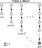
Figure 7.3: The backup digram for TD( )
. If
 , then the overall backup reduces to just its first component, the 1-step TD
backup, whereas, if
  , then the overall backup reduces to just its last
component, the Monte Carlo backup.
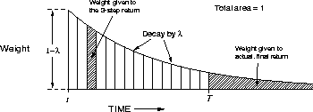
Figure 7.4: Weighting given in the  -return to each of the n
-step returns.
We define the  -return algorithm as the algorithm that performs
backups using the
  -return. On each step, t, it computes an increment,
 , to the value of the state occurring on that step:

(The increments for other states are of course  , for all
 .) Just as with the n
-step TD methods, the updating can be
either online or offline.
The approach that we have been taking so far is what we call the theoretical,
or forward, view of a learning algorithm. For each state visited, we look
forward in time to all the future rewards and decide how best to combine them.
We might imagine ourselves riding the stream of states, looking forward from each
state to determine its update, as suggested by Figure 7.5.
After looking forward from and updating one state, we move onto the next and
never have to work with the preceding state again. Future states, on the other
hand, are viewed and processed repeatedly, once from each vantage point preceding
them.

Figure 7.5: The forward or theoretical view. We decide how to update each
state by looking forward to future rewards and states.
The  -return algorithm is the basis for the forward view of eligibility
traces as used in the TD(
 )
method. In fact, we show in a later section that, in
the offline case, the
  -return algorithm is the TD(
 )
algorithm. The
 -return and TD(
 )
methods use the
  parameter to shift from 1-step TD methods
to Monte Carlo methods. The specific way this shift is done is interesting, but
not obviously better or worse than the way it is done with simple n
-step methods
by varying n
. Ultimately, the most compelling motivation for the
  way of
mixing n
-step backups is simply that there is a simple algorithm---TD(
 )
---for
achieving it. This is a mechanism issue rather than a theoretical one. In
the next few sections we develop the mechanistic, or backward, view of
eligibility traces as used in TD(
 )
.
)
.
Example  .
.
 -return on the Random Walk.
Figure 7.6 shows the performance of the offline
  -return
algorithm on the same 19-state random walk used with the n
-step methods in
Example 7.1. The experiment is just as in the n
-step case
except that here we vary
  instead of n
. Note that if
  is picked
appropriately then we get best performance with an intermediate value of
  .
.

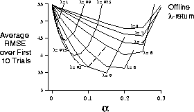
Figure 7.6: Performance of the offline  -return algorithm on a 19-state random-walk
task.
Exercise  .
.
The parameter  characterizes how fast the exponential weighting in
Figure 7.4 falls off, and thus how far into the future the
 -return algorithm looks in determining its backup. But a rate factor such as
 is sometimes an awkward way of characterizing the speed of the decay.
For some purposes it is better to specify a time constant, or half-life. What is
the formula for converting between
  and the half-life,
  ,
characterizing the time by which the weighting sequence will have fallen to
half of its initial value?


Next: 7.3 The Backward View
Up: 7 Eligibility Traces
Previous: 7.1 n-step TD Prediction
Richard Sutton
Fri May 30 15:01:47 EDT 1997
 . Any set of returns
can be averaged in this way, even an infinite set, as long as the weights on the
component returns are positive and sum to one. The overall return
possesses an error-correction property similar to that of individual n
-step
returns (7.2) and thus can be used to construct
backups with guaranteed convergence properties. Averaging produces a substantial
new range of algorithms. For example, one could average 1-step and infinite-step
backups to obtain another way of interrelating TD and Monte Carlo methods. In
principle, one could even average experience-based backups with DP backups to get
a simple combination of learning methods and model-based methods (see
Chapter 9
).


 )
algorithm can be understood as one particular way of averaging n
-step
backups. This average contains all the
n
-step backups, each weighted proportional to
  , where
  (Figure
  ensures that the
weights sum to 1. The resulting backup is toward a return, called the
 -return, defined by

 , the 2-step return the next
largest weight,
  , the 3-step return the weight
  , and so on,
the weight fading by
  with each additional step. After a terminal state
has been reached, all subsequent n
-step returns are equal to
  . If we
want, we can separate these terms from the main sum, yielding

 . In this case the main sum goes to zero, and the remaining term
reduces to the conventional return,
  . Thus, for
  , backing up
according to the
 -return is the same as the Monte Carlo algorithm that we called constant-
 \
MC (6.1) in the previous chapter. On the other hand, if
 , then the
  -return reduces to
  , the 1-step return. Thus, for
 , backing up according to the
  -return is the same as the 1-step TD
method, TD(0).

 )
. If
 , then the overall backup reduces to just its first component, the 1-step TD
backup, whereas, if
  , then the overall backup reduces to just its last
component, the Monte Carlo backup.
 -return to each of the n
-step returns.
 -return algorithm as the algorithm that performs
backups using the
  -return. On each step, t, it computes an increment,
 , to the value of the state occurring on that step:

 , for all
 .) Just as with the n
-step TD methods, the updating can be
either online or offline.

 -return algorithm is the basis for the forward view of eligibility
traces as used in the TD(
 )
method. In fact, we show in a later section that, in
the offline case, the
  -return algorithm is the TD(
 )
algorithm. The
 -return and TD(
 )
methods use the
  parameter to shift from 1-step TD methods
to Monte Carlo methods. The specific way this shift is done is interesting, but
not obviously better or worse than the way it is done with simple n
-step methods
by varying n
. Ultimately, the most compelling motivation for the
  way of
mixing n
-step backups is simply that there is a simple algorithm---TD(
 )
---for
achieving it. This is a mechanism issue rather than a theoretical one. In
the next few sections we develop the mechanistic, or backward, view of
eligibility traces as used in TD(
 )
.
)
.
 .
.
 -return on the Random Walk.
Figure
  -return
algorithm on the same 19-state random walk used with the n
-step methods in
Example 7.1. The experiment is just as in the n
-step case
except that here we vary
  instead of n
. Note that if
  is picked
appropriately then we get best performance with an intermediate value of
  .
.


 -return algorithm on a 19-state random-walk
task.
 .
.
 characterizes how fast the exponential weighting in
Figure
  -return algorithm looks in determining its backup. But a rate factor such as
 is sometimes an awkward way of characterizing the speed of the decay.
For some purposes it is better to specify a time constant, or half-life. What is
the formula for converting between
  and the half-life,
  ,
characterizing the time by which the weighting sequence will have fallen to
half of its initial value?