Our reason for computing the value function for a policy is to help
find better policies. Suppose we have determined the value function
![]() for an arbitrary deterministic policy
for an arbitrary deterministic policy ![]() . For some state
. For some state ![]() we
would like to know whether or not we should change the policy to
deterministically choose an action
we
would like to know whether or not we should change the policy to
deterministically choose an action
![]() . We know how good it is to follow the current
policy from
. We know how good it is to follow the current
policy from ![]() --that is
--that is ![]() --but would it be better or worse to
change to the new policy? One way to answer this question is to consider
selecting
--but would it be better or worse to
change to the new policy? One way to answer this question is to consider
selecting ![]() in
in ![]() and thereafter following the existing policy,
and thereafter following the existing policy, ![]() . The
value of this way of behaving is
. The
value of this way of behaving is
That this is true is a special case of a general result called the policy improvement theorem. Let ![]() and
and ![]() be any pair of
deterministic policies such that, for all
be any pair of
deterministic policies such that, for all ![]() ,
,
The idea behind the proof of the policy improvement theorem is easy to
understand. Starting from (4.7), we keep expanding the ![]() side and reapplying (4.7) until we get
side and reapplying (4.7) until we get ![]() :
:
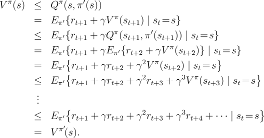
|
So far we have seen how, given a policy and its value function, we can easily
evaluate a change in the policy at a single state to a particular action.
It is a natural extension to consider changes at
all states and to all possible actions, selecting at each state
the action that appears best according to ![]() . In other words, to
consider the new greedy policy,
. In other words, to
consider the new greedy policy, ![]() , given by
, given by
Suppose the new greedy policy, ![]() , is as good as, but not better than, the old
policy
, is as good as, but not better than, the old
policy
![]() . Then
. Then ![]() , and from (4.9) it follows that for all
, and from (4.9) it follows that for all
![]() :
:
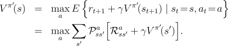
|
So far in this section we have considered the special case of deterministic
policies. In the general case, a stochastic policy ![]() specifies probabilities,
specifies probabilities,
![]() , for taking each action,
, for taking each action, ![]() , in each state,
, in each state, ![]() . We will not go
through the details, but in fact all the ideas of this section extend easily to
stochastic policies. In particular, the policy improvement theorem carries through
as stated for the stochastic case, under the natural definition:
. We will not go
through the details, but in fact all the ideas of this section extend easily to
stochastic policies. In particular, the policy improvement theorem carries through
as stated for the stochastic case, under the natural definition:
The last row of Figure
4.2 shows an example of policy
improvement for stochastic policies. Here the original policy, ![]() , is the
equiprobable random policy, and the new policy,
, is the
equiprobable random policy, and the new policy, ![]() , is greedy with respect to
, is greedy with respect to
![]() . The value function
. The value function ![]() is shown in the bottom-left diagram and the
set of possible
is shown in the bottom-left diagram and the
set of possible ![]() is shown in the bottom-right diagram. The states with
multiple arrows in the
is shown in the bottom-right diagram. The states with
multiple arrows in the ![]() diagram are those in which several actions
achieve the maximum in (4.9); any apportionment of probability
among these actions is permitted. The value function of any such policy,
diagram are those in which several actions
achieve the maximum in (4.9); any apportionment of probability
among these actions is permitted. The value function of any such policy,
![]() , can be seen by inspection to be either
, can be seen by inspection to be either ![]() ,
, ![]() , or
, or
![]() at all states,
at all states, ![]() , whereas
, whereas ![]() is at most
is at most ![]() . Thus,
. Thus,
![]() , for all
, for all ![]() , illustrating policy improvement.
Although in this case the new policy
, illustrating policy improvement.
Although in this case the new policy ![]() happens to be optimal, in general only
an improvement is guaranteed.
happens to be optimal, in general only
an improvement is guaranteed.