8.4 Control with Function Approximation

We now extend value-prediction methods using function approximation to control methods, following the pattern of GPI. First we extend the the state-value prediction methods to action-value prediction methods, then we combine them with policy-improvement and action-selection techniques. As usual, the problem of ensuring exploration is solved by pursuing either an on-policy or an off-policy approach.

The extension to action-value prediction is straightforward. In this case it is the action-value function, , that is represented as a parameterized functional form with parameter vector . Whereas before we considered training examples of the form , now we consider examples of the form . The example output, , can be any approximation of , including the usual backed-up values such as the full Monte-Carlo return, , or the 1-step Sarsa-style return, . The general gradient-descent update for action-value prediction is

For example, the backward view of the action-value method analogous to TD() is

where

and

with . We call this method gradient-descent Sarsa() , particularly when it is elaborated to form a full control method. For a constant policy, this method converges in the same way that TD() does, with the same kind of error bound (8.9).

To form control methods, we need to couple such action-value prediction methods with techniques for policy improvement and action selection. Suitable techniques applicable to continuous actions, or to actions from large discrete sets, are a topic of ongoing research with as yet no clear resolution. On the other hand, if the action set is discrete and not too large, then we can use the techniques already developed in previous chapters. That is, for each possible action, a, available in the current state, , we can compute and then find the greedy action . Policy improvement is done by changing the estimation policy to the greedy policy (in off-policy methods) or to a soft approximation of the greedy policy such as the -greedy policy (in on-policy methods). Actions are selected according to this same policy in on-policy methods, or by an arbitrary policy in off-policy methods.

Initialize  arbitrarily and 
Repeat (for each episode):
   
   For all :
      
      
   
   With probability : 
   Repeat (for each step of episode):
      
      For all : 	  (optional block for replacing traces)
          For all :
              
      For all :
          		      (accumulating traces)
          or                        (replacing traces)
      Take action a, observe reward, r, and next state, 
      
      For all :
         
         
      
      With probability : 
      
      
      
   until  is terminal

Initialize  arbitrarily and 
Repeat (for each episode):
   
   For all :
       
       
   Repeat (for each step of episode):
      With probability :
           
           
      else
           
           
      For all : 
      Take action a, observe reward, r, and next state, 
      
      For all :
         
         
      
      
      
   until  is terminal

Figures 8.8 and 8.9 show examples of on-policy (Sarsa() ) and off-policy (Watkins's Q() ) control methods using function approximation. Both methods use linear, gradient-descent function approximation with binary features, such as in tile coding and Kanerva coding. Both methods use an -greedy policy for action selection, and the Sarsa method uses it for GPI as well. Both compute the sets of present features, , corresponding to the current state and all possible actions, a. If the value function for each action is a separate linear function of the same features (a common case), then the indices of all the may be the same except for an offset, simplifying the computation significantly.

All the methods we have discussed above have used accumulating eligibility traces. Although replacing traces (Section 7.8) are known to have advantages in tabular methods, they do not directly extend to the use of function approximation. Recall that the idea of replacing traces is to reset a state's trace to 1 each time it is visited instead of incrementing it by 1. But with function approximation there is no single trace corresponding to a state, just a trace for each component of , each of which corresponds to many states. One approach that seems to work well for linear, gradient-descent function approximation with binary features is to treat the features as if they were states for the purposes of replacing traces. That is, each time a state is encountered that has feature i, the trace for feature i is set to 1 rather than being incremented by 1 as it would be with accumulating traces.

When working with state-action traces, it may also be useful to clear (set to zero) the traces of all non-selected actions in the states encountered (see Section 7.8). This idea can also be extended to the case of linear function approximation with binary features. For each state encountered, we first clear the traces of all features for the state and the actions not selected, then we set to 1 the traces of the features for the state and the action that was selected. As we noted for the tabular case, this may or may not be the best way to proceed when using replacing traces. A procedural specification of both kinds of traces, including the optional clearing for non-selected actions, is given for the Sarsa algorithm in Figure 8.8.

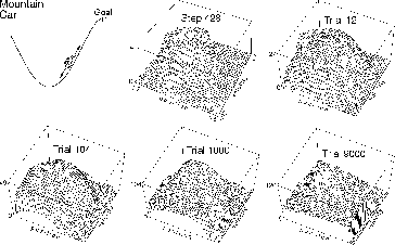
Example . The Mountain-Car Task. Consider the task of driving an underpowered car up a steep mountain road, as suggested by the diagram in the upper left of Figure 8.10. The difficulty is that gravity is stronger than the car's engine, and even at full throttle it cannot accelerate up the steep slope. The only solution is to first move away from the goal and up the opposite slope on the left. Then, by applying full throttle the car can build up enough inertia to carry it up the steep slope even though it is slowing down the whole way. This is a simple example of a continuous control task where things have to get worse in a sense (farther from the goal) before they can get better. Many control methodologies have great difficulties with tasks of this kind unless explicitly aided by a human designer.

  
Figure 8.10: The mountain-car task (upper left panel) and the cost-to-go function () learned during one run.

The reward in this problem is -1 on all time steps until the car has moved past its goal position at the top of the mountain, which ends the episode. There are three possible actions: full throttle forward (+1), full throttle reverse (-1), and zero throttle (0). The car moves according to a simplified physics. It's position, , and velocity, , are given by

where the bound operation enforces and . When reached the left bound, then was reset to zero. When it reached right bound, then the goal was reached and the episode was terminated. Each episode started from a random position and velocity uniformly chosen from these ranges. To convert the two continuous state variables to binary features, we used grid-tilings exactly as in Figure 8.5. We used ten tilings, each offset by a random fraction of a tile width.

The Sarsa algorithm in Figure 8.8 (using replace traces and the optional clearing) readily solved this task, learning a near optimal policy within 100 episodes. Figure 8.10 shows the negative of the value function (the cost-to-go function) learned on one run, using the parameters , , and (). The initial action values were all zero, which was optimistic (all true values are negative in this task), causing extensive exploration to occur even though the exploration parameter, , was 0. This can be seen in the middle-top panel of the figure, labeled ``Step 428." At this time not even one episode has been completed, but the car has oscillated back and forth in the valley, following circular trajectories in state space. All the states visited frequently are valued worse than unexplored states, because the actual rewards have been worse than what was (unrealistically) expected. This continually drives the agent away from wherever it has been to explore new states, until a solution is found. 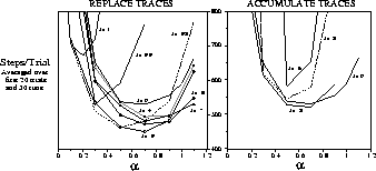Figure 8.11 shows the results of a detailed study of the effect of the parameters and , and of the kind of traces, on the rate of learning on this task.

  
Figure 8.11: The effect of , , and the kind of traces on early performance on the Mountain-Car task. This study used five tilings.

Exercise .*

Describe how the actor-critic control method could be combined with gradient-descent function approximation.