7.6 Q()

Two different methods have been proposed that combine eligibility traces and Q-learning, which we call Watkins's Q () and Peng's Q () after the researchers how first proposed them. First we describe Watkins's Q() .

Recall that Q-learning is an off-policy method, meaning that the policy learned about need not be the same as the one used to select actions. In particular, Q-learning learns about the greedy policy while it typically follows a policy involving exploratory actions---occasional selections of actions that are suboptimal according to . Because of this, special care is required when introducing eligibility traces.

Suppose we are backing up the state-action pair at time t. Suppose that on the successive two time steps the agent selects the greedy action, but on the third, at time t+3, the agent selects an exploratory, non-greedy action. In learning about the value of the greedy policy at we can only use subsequent experience as long as the greedy policy is being followed. Thus, we can use the 1-step and 2-step returns, but not in this case the 3-step return. The n -step returns for all no longer have any necessary relationship to the greedy policy.

Thus, unlike TD() or Sarsa() , Watkins's Q( ) does not look ahead all the way to the end of the episode in its backup. It only looks ahead as far as the next exploratory action. Aside from this difference, however, Watkins's Q( ) is much like TD() and Sarsa() . Their lookahead stops at episode's end, whereas Q( )'s lookahead stops at the first exploratory action, or at episode's end if there are no exploratory actions before that. Actually, to be more precise, 1-step Q-learning and Watkins's Q( ) both look one action past the first exploration, using their knowledge of the action values. For example, suppose the very first action, , is exploratory. Watkins's Q( ) would still do the one step update of toward . In general, if is the first exploratory action, then the longest backup is toward:

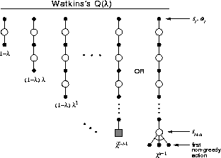
where here we assume offline updating. The backup diagram in Figure 7.13 illustrates the forward view of Watkins's Q( ), showing all the component backups.

  
Figure 7.13: The backup diagram for Watkins's Q( ). The series of component backups ends with either the end of the episode or the first non-greedy action, whichever comes first.

The mechanistic or backward view of Watkins's Q( ) is also very simple. Eligibility traces are used just as in Sarsa() , except that they are set to zero whenever an exploratory (non-greedy) action is taken. The trace update is best thought of as occurring in two steps. First, the traces for all state-action pairs are either decayed by or, if an exploratory action was taken, set to 0. Second, the trace corresponding to the current state and action is incremented by 1. The overall result is:

where, as before, is an identity-indicator function, equal to 1 if x=y and 0 otherwise. The rest of the algorithm is defined by:

where

Figure 7.14 shows the complete algorithm in pseudocode.

Initialize  arbitrarily and , for all s,a
Repeat (for each episode):
   Initialize s, a
   Repeat (for each step of episode):
      Take action a, observe r, 
      Choose  from  using policy derived from Q (e.g.,  -greedy)
       (if  ties for the max, then )
      
      
      For all s,a:
          
          If  then 
                     else 
      ; 
   until s is terminal

Unfortunately, cutting off traces every time an exploratory action is taken loses much of the advantage of using eligibility traces. If exploratory actions are frequent, as they often are early in learning, then only rarely will backups of more than one or two steps be done, and learning may be little faster than 1-step Q-learning. Peng's Q() is an alternate version of Q() meant to remedy this. Peng's Q() can be thought of as a hybrid of Sarsa() and Watkins's Q() .

  
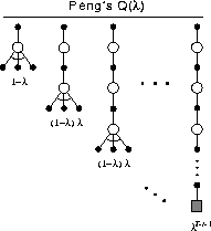
Figure 7.15: The backup diagram for Peng's Q() .

Conceptually, Peng's Q() uses the mixture of backups shown in Figure 7.15. Unlike Q-learning, there is no distinction between exploratory and greedy actions. Each component backup is over many steps of actual experiences, and all but the last is capped by a final maximization over actions. The component backups then are neither on-policy nor off-policy. The earlier transitions of each are on-policy whereas the last (fictitious) transition uses the greedy policy. As a consequence, for a fixed non-greedy policy, converges to neither nor under Peng's Q() algorithm, but to some hybrid of the two. However, if the policy is gradually made more greedy then the method may still converge to . As of this writing this has not yet been proved. Nevertheless, the method performs well empirically. Most studies have shown it performing significantly better than Watkins's Q() and almost as well as Sarsa() .

On the other hand, Peng's Q() can not be implemented as simply as Watkins's Q() . For a complete description of the needed implementation, see Peng and Williams (1994, 1996). One could imagine yet a third version of Q() , let us call it naive Q () , that is just like Watkins's Q() except that the traces are not set to zero on exploratory actions. This method might have some of the same advantages of Peng's Q() , but without the complex implementation. We know of no experience with this method, but perhaps it is not as naive as one might at first suppose.