First we consider how to compute the state-value function  for an
arbitrary policy,
for an
arbitrary policy,  . This is called policy evaluation in the DP
literature. We also refer to it as the prediction problem. Recall from
Chapter 3 that, for all
. This is called policy evaluation in the DP
literature. We also refer to it as the prediction problem. Recall from
Chapter 3 that, for all
 ,
,
where  is the probability of taking action a in state s under
policy
is the probability of taking action a in state s under
policy  , and the expectations are subscripted by
 to indicate that they are conditional on
  being followed. The
existence and uniqueness of
being followed. The
existence and uniqueness of  is guaranteed as long as either
 or eventual termination is guaranteed from all states under the
policy
or eventual termination is guaranteed from all states under the
policy  .
.
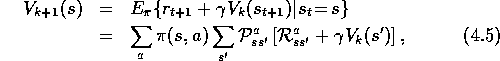
If the environment's dynamics are
completely known, then (4.4) is a system of  simultaneous
linear equations in
simultaneous
linear equations in
 unknowns (the
  ,
,  ). In principle, its solution is a
straightforward, if tedious, computation. For our purposes, iterative solution
methods are most suitable. Consider a sequence of approximate value functions
). In principle, its solution is a
straightforward, if tedious, computation. For our purposes, iterative solution
methods are most suitable. Consider a sequence of approximate value functions
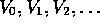 , each mapping
  to
to  . The initial
approximation,
. The initial
approximation,
 , is chosen arbitrarily (except that the terminal state, if any, must be
given value 0), and each successive approximation is obtained by using the
Bellman equation for
, is chosen arbitrarily (except that the terminal state, if any, must be
given value 0), and each successive approximation is obtained by using the
Bellman equation for  (3 .10
) as an update rule:
(3 .10
) as an update rule:
for all  .
Clearly,
.
Clearly,  is a fixed point for this update
rule because the Bellman equation for
is a fixed point for this update
rule because the Bellman equation for  assures us of equality in this
case. Indeed, the sequence
assures us of equality in this
case. Indeed, the sequence  can be shown in general to converge to
 as
as  under the same conditions that guarantee the
existence of
under the same conditions that guarantee the
existence of  . This algorithm is called iterative policy evaluation.
To produce each successive approximation,  from
from  , iterative policy
evaluation applies the same operation to each state s: it replaces the old value
of s with a new value obtained from the old values of the successor states of
s, and the expected immediate rewards, along all the one-step transitions
possible under the policy being evaluated. We call this kind of operation a
full backup. Each iteration of iterative policy evaluation backs
up the value of every state once to produce the new approximate value function
, iterative policy
evaluation applies the same operation to each state s: it replaces the old value
of s with a new value obtained from the old values of the successor states of
s, and the expected immediate rewards, along all the one-step transitions
possible under the policy being evaluated. We call this kind of operation a
full backup. Each iteration of iterative policy evaluation backs
up the value of every state once to produce the new approximate value function
 . There are several different kinds of full backups depending on whether
a state is being backed up (as here) or a state-action pair, and depending on the
precise way the estimated values of the successor states are combined. All the
backups done in DP algorithms are called full backups because they are
based on all possible next states rather than on a sample next state. The nature
of a backup can be expressed in an equation, as above, or in a backup diagram like
those introduced in Chapter 3. For example, Figure 3 .4
a is the
backup diagram corresponding to the full backup used in iterative policy
evaluation.
. There are several different kinds of full backups depending on whether
a state is being backed up (as here) or a state-action pair, and depending on the
precise way the estimated values of the successor states are combined. All the
backups done in DP algorithms are called full backups because they are
based on all possible next states rather than on a sample next state. The nature
of a backup can be expressed in an equation, as above, or in a backup diagram like
those introduced in Chapter 3. For example, Figure 3 .4
a is the
backup diagram corresponding to the full backup used in iterative policy
evaluation.
To write a sequential computer program to implement iterative policy evaluation, as
given by (4.5), you would have to use two arrays, one for
the old values,  , and one for the new values,
  . This way the
new values can be computed one by one from the old values without the
old values being changed. Of course it is easier simply to use one array and
update the values ``in place", that is, with each new backed-up value immediately
overwriting the old one. Then, depending on the order in which the states
are backed up, sometimes new values are used instead of old ones on the
righthand side of (4.5). This slightly different algorithm also
converges to
. This way the
new values can be computed one by one from the old values without the
old values being changed. Of course it is easier simply to use one array and
update the values ``in place", that is, with each new backed-up value immediately
overwriting the old one. Then, depending on the order in which the states
are backed up, sometimes new values are used instead of old ones on the
righthand side of (4.5). This slightly different algorithm also
converges to  ; in fact, it usually converges faster than the two-array
version, as you might expect since it uses new data as soon as it is available.
We think of the backups as being done in a sweep through the state space.
The order in which states are backed up during the sweep has a significant
influence on the rate of convergence. We usually have the in-place version in mind
when we think of DP algorithms.
; in fact, it usually converges faster than the two-array
version, as you might expect since it uses new data as soon as it is available.
We think of the backups as being done in a sweep through the state space.
The order in which states are backed up during the sweep has a significant
influence on the rate of convergence. We usually have the in-place version in mind
when we think of DP algorithms.
Another implementation point concerns the termination of the algorithm.
Formally, iterative policy evaluation converges only in the limit, but in practice
it must be halted short of this. A typical stopping condition for
iterative policy evaluation is to test the quantity 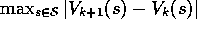 after each sweep and stop when it is sufficiently small.
Figure 4.1 gives a complete algorithm for
iterative policy evaluation with this stopping criterion.
after each sweep and stop when it is sufficiently small.
Figure 4.1 gives a complete algorithm for
iterative policy evaluation with this stopping criterion.
Input, the policy to be evaluated Initialize
, for all
Repeat
For each
:


until
(a small positive number) Output

Example  .
. Consider the
  gridworld shown below.

The nonterminal states are 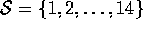 .
There are 4 actions possible in each state,
.
There are 4 actions possible in each state,  , which deterministically cause the corresponding state
transitions, except that actions that would take the agent off the grid in
fact leave the state unchanged. Thus, e.g.,
, which deterministically cause the corresponding state
transitions, except that actions that would take the agent off the grid in
fact leave the state unchanged. Thus, e.g.,  ,
,
 , and
, and  .
This is an undiscounted, episodic task. The reward
is -1 on all transitions until the terminal state is reached. The terminal
state is shaded in the figure (although it is shown in two places it
is formally one state). The expected reward
function is thus
.
This is an undiscounted, episodic task. The reward
is -1 on all transitions until the terminal state is reached. The terminal
state is shaded in the figure (although it is shown in two places it
is formally one state). The expected reward
function is thus  , for all states
  and actions a.
Suppose the agent follows the equiprobable random policy (all actions equally
likely). The left side of Figure 4.2 shows the sequence of value
functions
and actions a.
Suppose the agent follows the equiprobable random policy (all actions equally
likely). The left side of Figure 4.2 shows the sequence of value
functions  computed by iterative policy evaluation. The
final estimate is in fact
computed by iterative policy evaluation. The
final estimate is in fact  , which in this case gives for each state the
negation of the expected number of steps from that state until termination.
, which in this case gives for each state the
negation of the expected number of steps from that state until termination.

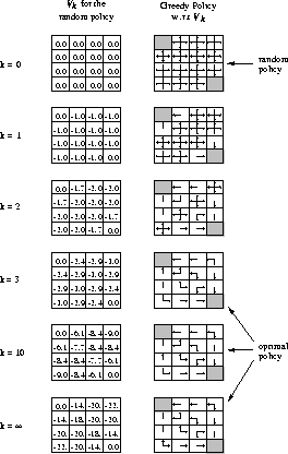
Figure 4.2: Convergence of iterative policy evaluation on a small gridworld. The
left column is the sequence of approximations of the value function for the
random policy (all actions equal). The right column is the
sequence of greedy policies corresponding to the value function estimates
(arrows are shown for all actions achieving the maximum).
The last policy is guaranteed only to be an improvement over the random
policy, but in this case it and all policies after the
third iteration are optimal.
Exercise  .
.
If  is the equiprobable random policy, what is
  ?
What is
?
What is  ?
?
Exercise  .
.
Suppose a new state 15 is added to the gridworld just below state 13, whose
actions, left, up, right, and down, take the agent to
states 12, 13, 14, and 15 respectively. Assume that the transitions from
the original states are unchanged. What then is  for the equiprobable
random policy? Now suppose the dynamics of state 13 are also changed, such that
action down from state 13 takes the agent to the new state 15. What is
for the equiprobable
random policy? Now suppose the dynamics of state 13 are also changed, such that
action down from state 13 takes the agent to the new state 15. What is
 for the equiprobable random policy in this case?
Exercise  .
.
What are the equations analogous to (4.3), (4.4) and
(4.5) for the action-value function
 and its successive approximation by a sequence of functions
  ?
?
Exercise  .
.
In some undiscounted episodic tasks there may be some policies for which
eventual termination is not guaranteed. For example, in the grid problem above
it is possible to go back and forth between two states forever. In a task that
is otherwise perfectly sensible,  may be negative infinity for some
policies and states, in which case the algorithm for iterative policy evaluation
given in Figure 4.1 will not terminate. As a purely
practical matter, how might we amend this algorithm to assure termination even in
this case. Assume that eventual termination is guaranteed under the
optimal policy.
may be negative infinity for some
policies and states, in which case the algorithm for iterative policy evaluation
given in Figure 4.1 will not terminate. As a purely
practical matter, how might we amend this algorithm to assure termination even in
this case. Assume that eventual termination is guaranteed under the
optimal policy.