The examples in the previous sections give some idea of the range of possibilities for combining methods of learning and planning. In the rest of this chapter, we analyze some of the component ideas involved, starting with the relative advantages of full and sample backups.
Much of this book has been about different kinds of backups, and we
have considered a great many varieties. Focusing for the moment on one-step
backups, they vary primarily along three binary
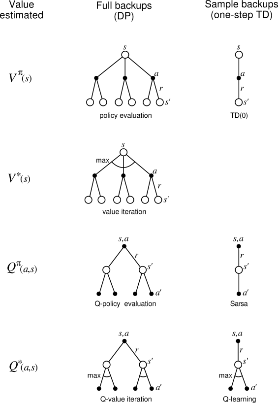
dimensions. The first two dimensions are whether they back up state values
or action values and whether they estimate the value for the optimal policy or
for an arbitrary given policy. These two dimensions give rise to four
classes of backups for approximating the four value functions, ![]() ,
, ![]() ,
,
![]() , and
, and ![]() . The other binary dimension is whether the backups are full backups, considering all possible events that might
happen, or sample backups, considering a single sample of what might
happen. These three binary dimensions give rise to eight cases, seven of which
correspond to specific algorithms, as shown in Figure
9.12.
(The eighth case does not seem to correspond to any useful backup.)
Any of these one-step backups can be used in planning methods. The
Dyna-Q agents discussed earlier use
. The other binary dimension is whether the backups are full backups, considering all possible events that might
happen, or sample backups, considering a single sample of what might
happen. These three binary dimensions give rise to eight cases, seven of which
correspond to specific algorithms, as shown in Figure
9.12.
(The eighth case does not seem to correspond to any useful backup.)
Any of these one-step backups can be used in planning methods. The
Dyna-Q agents discussed earlier use ![]() sample backups, but they could
just as well use
sample backups, but they could
just as well use ![]() full backups, or either full or sample
full backups, or either full or sample ![]() backups. The Dyna-AC system uses
backups. The Dyna-AC system uses ![]() sample backups together with a learning
policy structure. For stochastic problems, prioritized sweeping is always done
using one of the full backups.
sample backups together with a learning
policy structure. For stochastic problems, prioritized sweeping is always done
using one of the full backups.
When we introduced one-step sample backups in Chapter 6, we presented them as substitutes for full backups. In the absence of a distribution model, full backups are not possible, but sample backups can be done using sample transitions from the environment or a sample model. Implicit in that point of view is that full backups, if possible, are preferable to sample backups. But are they? Full backups certainly yield a better estimate because they are uncorrupted by sampling error, but they also require more computation, and computation is often the limiting resource in planning. To properly assess the relative merits of full and sample backups for planning we must control for their different computational requirements.
For concreteness, consider the full and sample backups for approximating ![]() , and
the special case of discrete states and actions, a table-lookup representation of
the approximate value function,
, and
the special case of discrete states and actions, a table-lookup representation of
the approximate value function, ![]() , and a model in the form of estimated
state-transition probabilities,
, and a model in the form of estimated
state-transition probabilities, ![]() , and expected rewards,
, and expected rewards, ![]() . The full backup for a state-action pair,
. The full backup for a state-action pair,
![]() , is:
, is:
The difference between these full and sample backups is significant to the
extent that the environment is stochastic, specifically, to the extent that,
given a state and action, many possible next states may occur with various
probabilities. If only one next state is possible, then the full and sample
backups given above are identical (taking ![]() ). If there are many possible
next states, then there may be significant differences. In favor of the full
backup is that it is an exact computation, resulting in a new
). If there are many possible
next states, then there may be significant differences. In favor of the full
backup is that it is an exact computation, resulting in a new ![]() whose
correctness is limited only by the correctness of the
whose
correctness is limited only by the correctness of the ![]() at successor
states. The sample backup is in addition affected by sampling error. On the other
hand, the sample backup is cheaper computationally because it considers only one
next state, not all possible next states. In practice, the computation required
by backup operations is usually dominated by the number of state-action pairs at
which
at successor
states. The sample backup is in addition affected by sampling error. On the other
hand, the sample backup is cheaper computationally because it considers only one
next state, not all possible next states. In practice, the computation required
by backup operations is usually dominated by the number of state-action pairs at
which ![]() is evaluated. For a particular starting pair,
is evaluated. For a particular starting pair, ![]() , let
, let ![]() be the
branching factor, the number of possible next states,
be the
branching factor, the number of possible next states, ![]() , for which
, for which ![]() . Then a full backup of this pair requires roughly
. Then a full backup of this pair requires roughly ![]() times as much
computation as a sample backup.
times as much
computation as a sample backup.
If there is enough time to complete a full backup, then the
resulting estimate is generally better than that of ![]() sample backups because of
the absence of sampling error. But if there is insufficient time to complete a full
backup, then sample backups are always preferable because they at least
make some improvement in the value estimate with fewer than
sample backups because of
the absence of sampling error. But if there is insufficient time to complete a full
backup, then sample backups are always preferable because they at least
make some improvement in the value estimate with fewer than ![]() backups. In a
large problem with many state-action pairs, we are often in the latter situation.
With so many state-action pairs, full backups of all of them would take a very long
time. Before that we may be much better off with a few sample backups at many
state-action pairs than with full backups at a few pairs. Given a unit of
computational effort, is it better devoted to a few full backups or to
backups. In a
large problem with many state-action pairs, we are often in the latter situation.
With so many state-action pairs, full backups of all of them would take a very long
time. Before that we may be much better off with a few sample backups at many
state-action pairs than with full backups at a few pairs. Given a unit of
computational effort, is it better devoted to a few full backups or to ![]() -times as
many sample backups?
-times as
many sample backups?
Figure
9.13 shows the results of an analysis that
suggests an answer to this question. It shows the estimation error as a function of
computation time for full and sample backups for a variety of branching factors,
![]() . The case considered is that in which all
. The case considered is that in which all ![]() successor states are equally
likely and in which the error in the initial estimate is 1. The values at the next
states are assumed correct, so the full backup reduces the error to zero upon its
completion. In this case, sample backups reduce the error according to
successor states are equally
likely and in which the error in the initial estimate is 1. The values at the next
states are assumed correct, so the full backup reduces the error to zero upon its
completion. In this case, sample backups reduce the error according to
![]() where
where ![]() is the number of sample backups that have
been performed (assuming sample averages, i.e.,
is the number of sample backups that have
been performed (assuming sample averages, i.e., ![]() ). The key observation
is that for moderately large
). The key observation
is that for moderately large ![]() the error falls dramatically with a tiny fraction
of
the error falls dramatically with a tiny fraction
of ![]() backups. For these cases, many state-action pairs could have their values
improved dramatically, to within a few percent of the effect of a full backup, in
the same time that one state-action pair could be backed up fully.
backups. For these cases, many state-action pairs could have their values
improved dramatically, to within a few percent of the effect of a full backup, in
the same time that one state-action pair could be backed up fully.
The advantage of sample backups shown in Figure 9.13 is probably an underestimate of the real effect. In a real problem, the values of the successor states would themselves be estimates updated by backups. By causingestimates to be more accurate sooner, sample backups will have a second advantage in that the values backed up from the successor states will be more accurate. These results suggest that sample backups are likely to be superior to full backups on problems with large stochastic branching factors and too many states to be solved exactly.
Exercise 9.5 The analysis above assumed that all of the