Backups can be done not just toward any ![]() -step return, but toward any average of
-step return, but toward any average of ![]() -step returns. For example, a backup can be done toward a return
that is half of a two-step return and half of a four-step return:
-step returns. For example, a backup can be done toward a return
that is half of a two-step return and half of a four-step return:
![]() . Any set of returns
can be averaged in this way, even an infinite set, as long as the weights on the
component returns are positive and sum to 1. The overall return
possesses an error reduction property similar to that of individual
. Any set of returns
can be averaged in this way, even an infinite set, as long as the weights on the
component returns are positive and sum to 1. The overall return
possesses an error reduction property similar to that of individual ![]() -step
returns (7.2) and thus can be used to construct
backups with guaranteed convergence properties. Averaging produces a substantial
new range of algorithms. For example, one could average one-step and infinite-step
backups to obtain another way of interrelating TD and Monte Carlo methods. In
principle, one could even average experience-based backups with DP backups to get
a simple combination of experience-based and model-based methods (see
Chapter 9).
-step
returns (7.2) and thus can be used to construct
backups with guaranteed convergence properties. Averaging produces a substantial
new range of algorithms. For example, one could average one-step and infinite-step
backups to obtain another way of interrelating TD and Monte Carlo methods. In
principle, one could even average experience-based backups with DP backups to get
a simple combination of experience-based and model-based methods (see
Chapter 9).
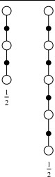
A backup that averages simpler component backups in this way is called a complex backup. The backup diagram for a complex backup consists of the backup diagrams for each of the component backups with a horizontal line above them and the weighting fractions below. For example, the complex backup mentioned above, mixing half of a two-step backup and half of a four-step backup, has the diagram:
|
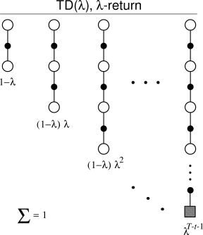
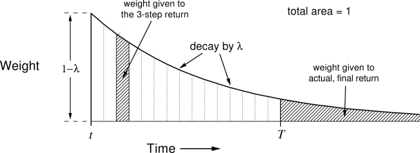
The TD(![]() ) algorithm can be understood as one particular way of averaging
) algorithm can be understood as one particular way of averaging ![]() -step
backups. This average contains all the
-step
backups. This average contains all the
![]() -step backups, each weighted proportional to
-step backups, each weighted proportional to ![]() , where
, where ![]() (Figure
7.3). A normalization factor of
(Figure
7.3). A normalization factor of ![]() ensures that the
weights sum to 1. The resulting backup is toward a return, called the
ensures that the
weights sum to 1. The resulting backup is toward a return, called the ![]() -return, defined by
-return, defined by
|
We define the ![]() -return algorithm as the algorithm that performs
backups using the
-return algorithm as the algorithm that performs
backups using the ![]() -return. On each step,
-return. On each step, ![]() , it computes an increment,
, it computes an increment,
![]() , to the value of the state occurring on that step:
, to the value of the state occurring on that step:
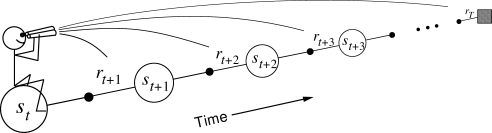
The approach that we have been taking so far is what we call the theoretical, or forward, view of a learning algorithm. For each state visited, we look forward in time to all the future rewards and decide how best to combine them. We might imagine ourselves riding the stream of states, looking forward from each state to determine its update, as suggested by Figure 7.5. After looking forward from and updating one state, we move on to the next and never have to work with the preceding state again. Future states, on the other hand, are viewed and processed repeatedly, once from each vantage point preceding them.
|
The ![]() -return algorithm is the basis for the forward view of eligibility
traces as used in the TD(
-return algorithm is the basis for the forward view of eligibility
traces as used in the TD(![]() ) method. In fact, we show in a later section that, in
the off-line case, the
) method. In fact, we show in a later section that, in
the off-line case, the ![]() -return algorithm is the TD(
-return algorithm is the TD(![]() ) algorithm. The
) algorithm. The
![]() -return and TD(
-return and TD(![]() ) methods use the
) methods use the ![]() parameter to shift from one-step TD methods
to Monte Carlo methods. The specific way this shift is done is interesting, but
not obviously better or worse than the way it is done with simple
parameter to shift from one-step TD methods
to Monte Carlo methods. The specific way this shift is done is interesting, but
not obviously better or worse than the way it is done with simple ![]() -step methods
by varying
-step methods
by varying ![]() . Ultimately, the most compelling motivation for the
. Ultimately, the most compelling motivation for the ![]() way of
mixing
way of
mixing ![]() -step backups is that there is a simple algorithm--TD(
-step backups is that there is a simple algorithm--TD(![]() )--for
achieving it. This is a mechanism issue rather than a theoretical one. In
the next few sections we develop the mechanistic, or backward, view of
eligibility traces as used in TD(
)--for
achieving it. This is a mechanism issue rather than a theoretical one. In
the next few sections we develop the mechanistic, or backward, view of
eligibility traces as used in TD(![]() ).
).
Example 7.2:

Exercise 7.4 The parameter