

Next: 6.3 Optimality of TD(0)
Up: 6 Temporal Difference Learning
Previous: 6.1 TD Prediction
TD methods learn their estimates in part on the basis of other estimates. They
learn a guess from a guess---they bootstrap. Is this a good thing to do?
What advantages do TD methods have over Monte Carlo and DP methods? Developing and
answering such questions will take the rest of this book and more. In this section
we briefly anticipate some of the answers.
Obviously, TD methods have an advantage over DP methods in that they do not
require a model of the environment, of its reward and next-state probability
distributions.
The next most obvious advantage of TD methods over Monte Carlo methods is that
they are naturally implemented in an online, fully incremental fashion. With
Monte Carlo methods one must wait until the end of an episode, because only then
is the return known, whereas with TD methods one need only wait one time step.
Surprisingly often this turns out to be a critical consideration. Some
applications have very long episodes, so that delaying all learning until an
episode's end is just too slow. Other applications are continual and have no
episodes at all. Finally, as we noted in the previous chapter, some Monte Carlo
methods must ignore or discount episodes on which experimental actions are
taken, which can greatly slow learning. TD methods are much less susceptible to
these problems because they learn from each transition regardless of what
subsequent actions are taken.
But are TD methods sound? Certainly it is convenient to learn one guess from the
next, without waiting for an actual outcome, but can we still guarantee
convergence to the correct answer? Happily, the answer is yes. For any fixed
policy  , the TD algorithm described above has been proven to converge to
 , in the mean for a constant step-size parameter if it is sufficiently small,
and with probability one if the step-size parameter decreases according to the
usual stochastic approximation conditions (
 ). Most
convergence proofs apply only to the table-based case of the algorithm presented
above (6.2), but some also apply to the case of general linear function
approximators. These results are discussed in a more general setting in the
next two chapters.
If both TD and MC methods converge asymptotically to the correct predictions, then
a natural next question is ``Which gets there first?" In other words, which
method learns fastest? Which makes the most efficient use of limited data? At
the current time this is an open question in the sense that no one has been able
to prove mathematically that one method converges faster than the other. In
fact, it is not even clear what is the most appropriate formal way to phrase
this question! In practice, however, TD methods have usually been found to
converge faster than MC methods on stochastic tasks, as illustrated in the
following example.
Example  .
. Random Walk.
In this example we empirically compare the prediction
abilities of TD(0) and constant-
 MC applied to the small Markov
process shown in Figure 6.5. All episodes start in
the center state, C, and proceed either left or right by one state on
each step, with equal probability. This behavior is presumably due to the
combined effect of a fixed policy and an environment's state-transition
probabilities, but we do not care which; we are concerned only with predicting
returns however they are generated. Episodes terminate either on the extreme left
or the extreme right. If they terminate on the right a reward of +1 occurs,
and otherwise all rewards are zero. For example, a typical walk might consist of the
following state-and-reward sequence:
C,0,B,0,C,0,D,0,E,1. Because this task is undiscounted and episodic, the
true value of each state is just the probability of terminating on the right if
starting from that state. Thus, the true value of the center state is
 . The true values of all the states, A through E, are
  , and
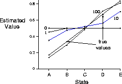
, and  . Figure 6.6
shows the values learned by TD(0) approaching the true values as
more episodes are experienced. Averaging over many episode sequences,
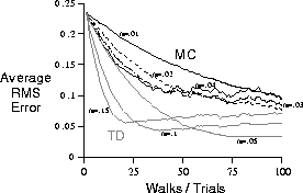
Figure 6.7 shows the average error in the predictions found by
TD(0) and constant-
 MC, for a variety of values of
  , as a function of number of
episodes. In all cases the approximate value function was initialized to the
intermediate value
 , for all s. The TD method is consistently better than the MC method on this task
over this number of episodes.


Figure 6.5: A small Markov process for generating random walks. Walks start in
the center, then move randomly right or left until entering a terminal state.
Termination on the right produces a reward of +1; all other transitions yield
zero reward.

Figure 6.6: Values learned by TD(0) after various numbers of episodes. The final
estimate is about as close as the estimates ever get to the true values. With a
constant step-size parameter ( in this example), the values fluctuate
indefinitely in response to the outcomes of the most recent episodes.

Figure 6.7: Learning curves for TD(0) and constant- MC methods, for various values
of
  , on the prediction problem for the random walk. The performance
measure shown is the squared error between the value function learned and the true
value function, averaged over the five states. These data are averages over 100
different sequences of episodes.
Exercise  .
.
This is a exercise to help develop your intuition about why TD
methods are often more efficient than MC methods. Consider the driving-home example
and how it is addressed by TD and MC methods. Can you imagine a scenario in which a
TD update would be better on average than an MC update? Give an example scenario---a
description of past experience and a current situation---in which you would expect
the TD update to be better.
Here's a hint: Suppose you have
lots of experience driving home from work. Then you move to a new
building and a new parking lot (but you still enter the highway at
the same place). Now you are starting to learn predictions for the new
building. Can you see why TD updates are likely to be much better, at
least initially, in this case? Might the same sort of thing happen in
the original task?
Exercise  .
.
From Figure 6.6, it appears that the first episode results in a change in
only  . What does this tell you about what happened on the first
episode? Why was only the estimate for this one state changed? By exactly how much
was it changed?
Exercise  .
.
Do you think that by choosing the step-size parameter,  , differently,
either algorithm could have done significantly better than shown in
Figure 6.7? Why or why not?
Exercise  .
.
In Figure 6.7, the RMS error of the TD method seems to go
down and then up again, particularly at high  's. What could have caused this? Do
you think this always occurs, or might it be a function of how the approximate
value function was initialized?
Exercise  .
.
Above we stated that the true values for the random walk task are  , and
, and  , for states A through
E. Describe at least two different ways that these could have been computed.
Which would you guess we actually used? Why?


Next: 6.3 Optimality of TD(0)
Up: 6 Temporal Difference Learning
Previous: 6.1 TD Prediction
Richard Sutton
Fri May 30 13:53:05 EDT 1997
 , the TD algorithm described above has been proven to converge to
 , in the mean for a constant step-size parameter if it is sufficiently small,
and with probability one if the step-size parameter decreases according to the
usual stochastic approximation conditions (
 ). Most
convergence proofs apply only to the table-based case of the algorithm presented
above (6.2), but some also apply to the case of general linear function
approximators. These results are discussed in a more general setting in the
next two chapters.


 .
. Random Walk.
In this example we empirically compare the prediction
abilities of TD(0) and constant-
 MC applied to the small Markov
process shown in Figure
  . The true values of all the states, A through E, are
  , and
, and  . Figure
  MC, for a variety of values of
  , as a function of number of
episodes. In all cases the approximate value function was initialized to the
intermediate value
 , for all s. The TD method is consistently better than the MC method on this task
over this number of episodes.


 in this example), the values fluctuate
indefinitely in response to the outcomes of the most recent episodes.
 MC methods, for various values
of
  , on the prediction problem for the random walk. The performance
measure shown is the squared error between the value function learned and the true
value function, averaged over the five states. These data are averages over 100
different sequences of episodes.
 .
.
 .
.
 . What does this tell you about what happened on the first
episode? Why was only the estimate for this one state changed? By exactly how much
was it changed?
 .
.
 , differently,
either algorithm could have done significantly better than shown in
Figure
  .
.
 's. What could have caused this? Do
you think this always occurs, or might it be a function of how the approximate
value function was initialized?
 .
.
 , and
, and  , for states A through
E. Describe at least two different ways that these could have been computed.
Which would you guess we actually used? Why?