

Next: 8.3.2 Tile Coding
Up: 8.3 Linear Methods
Previous: 8.3 Linear Methods
Consider a task in which the state set is continuous and two-dimensional.
A state in this case consists of a point in two-space, say a vector with two real
components. One kind of feature for this case are
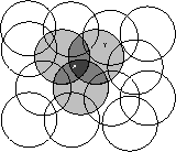
those corresponding to circles in state space, as shown in
Figure 8.2. If the state is inside a circle, then the
corresponding feature has the value 1 and is said to be
present; otherwise the feature is 0 and is said to be
absent. This kind of 1-0 valued feature is called a binary feature.
Given a state, which binary features are present indicate within
which circles the state lies, and thus coarsely code for its location.
Representing a state with features that overlap in this way
(although they need not be circles or binary) is known as coarse coding.

Figure 8.2: Coarse coding. Generalization from state X to state Y depends on the
number of their features whose receptive fields (in this case,
circles) overlap. These states have one feature in common, so
there will be slight generalization between them.
Assuming a linear gradient-descent function approximator, consider the
effect of the size and density of the circles. Corresponding to each circle is
a single parameter (a component of  ) that is affected by learning. If we
train at one point (state),
X, then the parameters of all circles intersecting
X will be affected. Thus, by (8.8), the approximate value
function will be affected at all points within the union of the circles,
with a greater effect the more circles a point has ``in common" with X, as
shown in Figure 8.2. If the circles are small,
then the generalization will be over a short distance, as in
Figure 8.3a, whereas if they are large, it will be over a
large distance, as in
Figure 8.3b. Moreover, the shape of the features will
determine the nature of the generalization. For example, if they are not
strictly circular, but are elongated in one direction, then generalization
will be similarly affected, as in Figure 8.3c.

Figure 8.3: Generalization in linear function approximators is determined by the
sizes and shapes of the features' receptive fields. All three of these
cases have roughly the same number and density of features.
Features with large receptive fields give broad generalization, but might
also seem to limit the learned function to a coarse approximation, unable to
make discriminations much finer than the width of the receptive fields.
Happily, this is not the case. Initial generalization from one point to
another is indeed controlled by the size and shape of the receptive
fields, but acuity, the finest discrimination ultimately possible, is
controlled more by the total number of features.
Example  .
. The Coarseness of Coarse Coding.
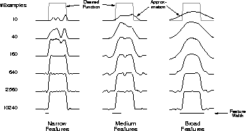
This example illustrates the effect on learning of the size of the receptive
fields in coarse coding. A linear function
approximator based on coarse coding and (8.3) was used to
learn a one-dimensional square-wave function (shown at the top of
Figure 8.4). The values of this function were used as the targets,
 . With just one dimension,
the receptive fields were intervals rather than circles. Learning was
repeated with three different sizes of the intervals: narrow, medium, and broad,
as shown at the bottom of the figure. All three cases had the same density of
features, about 50 over the extent of the function being learned. Training
examples were generated uniformly at random over this extent. The
step-size parameter was
 , where m is the number of features that were present at
one time. Figure 8.4 shows the functions learned in all
three cases over the course of learning. Note that the width of the features
had a strong effect early in learning. With broad features, the
generalization tended to be broad; with narrow features, only the close
neighbors of each trained point were changed, causing the function learned
to be more bumpy. However, the final function learned was affected only
slightly by the width of the features. Receptive field shape tends to have
a strong effect on generalization, but little effect on asymptotic solution
quality.


Figure 8.4: Example of feature width's strong effect on initial
generalization (first row) and weak effect on asymptotic accuracy (last row).


Next: 8.3.2 Tile Coding
Up: 8.3 Linear Methods
Previous: 8.3 Linear Methods
Richard Sutton
Sat May 31 15:08:20 EDT 1997


 ) that is affected by learning. If we
train at one point (state),
X, then the parameters of all circles intersecting
X will be affected. Thus, by (
 .
. The Coarseness of Coarse Coding.
This example illustrates the effect on learning of the size of the receptive
fields in coarse coding. A linear function
approximator based on coarse coding and (
 . With just one dimension,
the receptive fields were intervals rather than circles. Learning was
repeated with three different sizes of the intervals: narrow, medium, and broad,
as shown at the bottom of the figure. All three cases had the same density of
features, about 50 over the extent of the function being learned. Training
examples were generated uniformly at random over this extent. The
step-size parameter was
 , where m is the number of features that were present at
one time. Figure
