 , is
, is


A reinforcement learning task that satisfies the Markov property is called a Markov decision process, or MDP. If the state and action spaces are finite, then it is called a finite Markov decision process (finite MDP). Finite MDPs are particularly important to the theory of reinforcement learning. We treat them extensively throughout this book; they are all you need to understand for 90% of modern reinforcement learning.
A particular finite MDP is defined by its state and action sets and by the one-step
dynamics of the environment. Given any state and action, s and
a, the probability of each possible next state,  , is
, is
Similarly, given any current state and action, s and a, together with any
next state,  , the expected value of the next reward is
These two quantities,  and
and  , completely specify the
most important aspects of the dynamics of a finite MDP (only information about the
distribution of rewards around the expected value is lost). Most of the theory we present in the rest of this book
implicitly assumes the environment is a finite MDP.
Example  .
.
Recycling Robot MDP. The recycling robot (Example 3.3) can be turned into a simple example of an MDP by simplifying it and providing some more details. (Our aim is to produce a simple example, not a particularly realistic one.) Recall that the agent makes a decision at times determined by external events (or by other parts of the robot's control system). At each such time the robot decides whether it should 1) actively search for a can, 2) remain stationary and wait for someone to bring it a can, or 3) go back to home base to recharge its battery. Suppose the environment works as follows. The best way to find cans is to actively search for them, but this runs down the robot's battery, whereas just waiting does not. Whenever the robot is searching, the possibility exists that its battery will become depleted. In this case the robot must shut down and wait to be rescued (producing a low reward).
The agent makes its decisions solely on the basis of the energy level of the
battery. It can distinguish two levels, high and
low, so that the state set is  . Let us
call the possible decisions---the agent's actions--- wait, search, and
recharge. When the energy level is high, recharging would always be
foolish, so we do not include it in the action set for this state. The agent's
action sets are:

If the energy level is high, then a period of active search
can always be completed without risk of depleting the battery. A period of searching
beginning with a high energy level leaves the energy level high with
probability  and reduces it to low with probability
  . On the
other hand, a period of searching undertaken when the energy level is low
leaves it low with probability
  and depletes the battery with probability
 . In the latter case, the robot must be rescued, but then the battery is then
recharged back to high. Each can collected by the robot counts as a unit reward,
whereas a reward of -3 results whenever the robot has to be rescued. Let
 and
and
 , with
  , respectively denote the expected
number of cans the robot will collect (and hence the expected reward) while
searching and while waiting. Finally, to keep things simple, suppose that no cans
can be collected during a run home for recharging, and that no cans can be collected
on a step in which the battery is depleted. This system is then a finite MDP, and
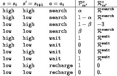
we can write down the transition probabilities and the expected rewards, as in
Table 3.1.

Table 3.1: Transition probabilities and expected rewards for the finite
MDP of the recycling-robot example. There is a row for each
possible combination of current state, s, next state, , and action possible
in the current state,
  .
.
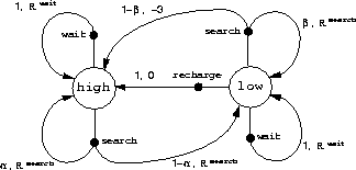
A transition graph is a useful way to summarize the dynamics of a
finite MDP.
Figure 3.3 shows the transition graph for the recycling robot
example. There are two kinds of nodes: state nodes and
action nodes. There is a state node for each possible state (a large
open circle labeled by the name of the state), and an action node for each
state-action pair  (a small solid circle labeled
by a and connected by a line to the state node s). Starting in state s and
taking action a moves you along the line from state node s to
action node
  . Then the environment responds with a transition to the
next state's node via one of the arrows leaving action node
  . Each arrow
corresponds to a triple
  , where
  is the next state, and we label
the arrow with the transition probability,
  , and the expected
reward for that transition,
 . Note that the transition probabilities labeling the
arrows leaving an action node always sum to one.

Figure 3.3: Transition graph for the recycling-robot example. The graph has a
node for each state, shown as a large circle, and a node for each state-action pair,
shown as a small solid circle. Each arrow is labeled by the transition
probability and the expected reward for that transition.

Exercise  .
.
Assuming a finite MDP with a finite number of reward values, write an equation for the transition probabilities and the expected rewards in terms of the joint conditional distribution in (3.5).


