We turn now to the use of TD prediction methods for the control problem. As usual, we follow the pattern of generalized policy iteration (GPI), only this time using TD methods for the evaluation or prediction part. As with Monte Carlo methods, we face the need to trade off exploration and exploitation, and again approaches fall into two main classes: on-policy and off-policy. In this section we present an on-policy TD control method.
The first step is to learn an action-value function rather than a state-value
function. In particular, for an on-policy method we must estimate ![]() for the current behavior policy
for the current behavior policy ![]() and for all states
and for all states ![]() and actions
and actions ![]() .
This can be done using essentially the same TD method
described above for learning
.
This can be done using essentially the same TD method
described above for learning ![]() . Recall that an episode consists of an
alternating sequence of states and state-action pairs:
. Recall that an episode consists of an
alternating sequence of states and state-action pairs:
It is straightforward to design an on-policy control algorithm based on the
Sarsa prediction method. As in all on-policy methods, we continually estimate
![]() for the behavior policy
for the behavior policy ![]() , and at the same time change
, and at the same time change ![]() toward
greediness with respect to
toward
greediness with respect to ![]() . The general form of the Sarsa control
algorithm is given in Figure
6.9.
. The general form of the Sarsa control
algorithm is given in Figure
6.9.
The convergence properties of the Sarsa algorithm depend on the
nature of the policy's dependence on ![]() . For example, one could use
. For example, one could use ![]() -greedy or
-greedy or
![]() -soft policies. According to Satinder Singh (personal communication), Sarsa
converges with probability
-soft policies. According to Satinder Singh (personal communication), Sarsa
converges with probability ![]() to an optimal policy and action-value function as long
as all state-action pairs are visited an infinite number of times and the policy
converges in the limit to the greedy policy (which can be arranged, for example,
with
to an optimal policy and action-value function as long
as all state-action pairs are visited an infinite number of times and the policy
converges in the limit to the greedy policy (which can be arranged, for example,
with ![]() -greedy policies by setting
-greedy policies by setting ![]() ), but this result has not yet been
published in the literature.
), but this result has not yet been
published in the literature.
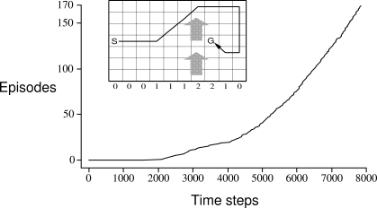
Example 6.5: Windy Gridworld Figure 6.10 shows a standard gridworld, with start and goal states, but with one difference: there is a crosswind upward through the middle of the grid. The actions are the standard four--up, down, right, and left--but in the middle region the resultant next states are shifted upward by a "wind," the strength of which varies from column to column. The strength of the wind is given below each column, in number of cells shifted upward. For example, if you are one cell to the right of the goal, then the action left takes you to the cell just above the goal. Let us treat this as an undiscounted episodic task, with constant rewards of

Exercise 6.6: Windy Gridworld with King's Moves Resolve the windy gridworld task assuming eight possible actions, including the diagonal moves, rather than the usual four. How much better can you do with the extra actions? Can you do even better by including a ninth action that causes no movement at all other than that caused by the wind?
Exercise 6.7: Stochastic Wind Resolve the windy gridworld task with King's moves, assuming that the effect of the wind, if there is any, is stochastic, sometimes varying by 1 from the mean values given for each column. That is, a third of the time you move exactly according to these values, as in the previous exercise, but also a third of the time you move one cell above that, and another third of the time you move one cell below that. For example, if you are one cell to the right of the goal and you move left, then one-third of the time you move one cell above the goal, one-third of the time you move two cells above the goal, and one-third of the time you move to the goal.
Exercise 6.8 What is the backup diagram for Sarsa?