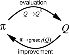
We are now ready to consider how Monte Carlo estimation can be used in control, that is, to approximate optimal policies. The overall idea is to proceed according to the same pattern as in the DP chapter, that is, according to the idea of generalized policy iteration (GPI). In GPI one maintains both an approximate policy and an approximate value function. The value function is repeatedly altered to more closely approximate the value function for the current policy, and the policy is repeatedly improved with respect to the current value function:
|
To begin, let us consider a Monte Carlo version of classical policy iteration.
In this method, we perform alternating complete
steps of policy evaluation and policy improvement, beginning with an arbitrary
policy ![]() and ending with the optimal policy and optimal action-value
function:
and ending with the optimal policy and optimal action-value
function:
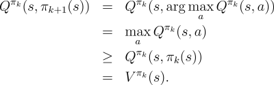
Policy improvement is done by making the policy greedy with respect
to the current value function. In this case we have an action-value
function, and therefore no model is needed to construct the greedy policy.
For any action-value function ![]() , the corresponding greedy policy is the one
that, for each
, the corresponding greedy policy is the one
that, for each
![]() , deterministically chooses an action with maximal
, deterministically chooses an action with maximal ![]() -value:
-value:
|
We made two unlikely assumptions above in order to easily obtain this guarantee of convergence for the Monte Carlo method. One was that the episodes have exploring starts, and the other was that policy evaluation could be done with an infinite number of episodes. To obtain a practical algorithm we will have to remove both assumptions. We postpone consideration of the first assumption until later in this chapter.
For now we focus on the assumption that policy evaluation operates on
an infinite number of episodes. This assumption is relatively easy
to remove. In fact, the same issue arises even in classical DP methods
such as iterative policy evaluation, which also converge only asymptotically to
the true value function. In both DP and Monte Carlo cases there are two
ways to solve the problem. One is to hold firm to the idea of approximating
![]() in each policy evaluation. Measurements and assumptions
are made to obtain bounds on the magnitude and probability of error in the
estimates, and then sufficient steps are taken during each policy evaluation
to assure that these bounds are sufficiently small. This approach can
probably be made completely satisfactory in the sense
of guaranteeing correct convergence up to some level of approximation.
However, it is also likely to require far too many episodes to be useful in
practice on any but the smallest problems.
in each policy evaluation. Measurements and assumptions
are made to obtain bounds on the magnitude and probability of error in the
estimates, and then sufficient steps are taken during each policy evaluation
to assure that these bounds are sufficiently small. This approach can
probably be made completely satisfactory in the sense
of guaranteeing correct convergence up to some level of approximation.
However, it is also likely to require far too many episodes to be useful in
practice on any but the smallest problems.
The second approach to avoiding the infinite number of episodes nominally
required for policy evaluation is to forgo trying to complete policy
evaluation before returning to policy improvement. On each evaluation step
we move the value function toward ![]() , but we do not expect
to actually get close except over many steps. We used this idea when
we first introduced the idea of GPI in Section 4.6. One extreme form of
the idea is value iteration, in which only one iteration of iterative policy
evaluation is performed between each step of policy improvement. The
in-place version of value iteration is even more extreme; there we alternate
between improvement and evaluation steps for single states.
, but we do not expect
to actually get close except over many steps. We used this idea when
we first introduced the idea of GPI in Section 4.6. One extreme form of
the idea is value iteration, in which only one iteration of iterative policy
evaluation is performed between each step of policy improvement. The
in-place version of value iteration is even more extreme; there we alternate
between improvement and evaluation steps for single states.
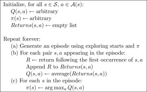
For Monte Carlo policy evaluation it is natural to alternate between evaluation and improvement on an episode-by-episode basis. After each episode, the observed returns are used for policy evaluation, and then the policy is improved at all the states visited in the episode. A complete simple algorithm along these lines is given in Figure 5.4. We call this algorithm Monte Carlo ES, for Monte Carlo with Exploring Starts.
In Monte Carlo ES, all the returns for each state-action pair are accumulated and averaged, irrespective of what policy was in force when they were observed. It is easy to see that Monte Carlo ES cannot converge to any suboptimal policy. If it did, then the value function would eventually converge to the value function for that policy, and that in turn would cause the policy to change. Stability is achieved only when both the policy and the value function are optimal. Convergence to this optimal fixed point seems inevitable as the changes to the action-value function decrease over time, but has not yet been formally proved. In our opinion, this is one of the most fundamental open questions in reinforcement learning.
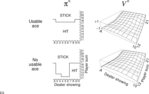
Example 5.3: Solving Blackjack It is straightforward to apply Monte Carlo ES to blackjack. Since the episodes are all simulated games, it is easy to arrange for exploring starts that include all possibilities. In this case one simply picks the dealer's cards, the player's sum, and whether or not the player has a usable ace, all at random with equal probability. As the initial policy we use the policy evaluated in the previous blackjack example, that which sticks only on 20 or 21. The initial action-value function can be zero for all state-action pairs. Figure 5.5 shows the optimal policy for blackjack found by Monte Carlo ES. This policy is the same as the "basic" strategy of Thorp (1966) with the sole exception of the leftmost notch in the policy for a usable ace, which is not present in Thorp's strategy. We are uncertain of the reason for this discrepancy, but confident that what is shown here is indeed the optimal policy for the version of blackjack we have described.