7.4 Equivalence of Forward and Backward Views

In this section we show that off-line TD($\lambda$), as defined mechanistically above, achieves the same weight updates as the off-line $\lambda$-return algorithm. In this sense we align the forward (theoretical) and backward (mechanistic) views of TD($\lambda$). Let denote the update at time of according to the $\lambda$-return algorithm (7.4), and let denote the update at time of state according to the mechanistic definition of TD($\lambda$) as given by (7.7). Then our goal is to show that the sum of all the updates over an episode is the same for the two algorithms:

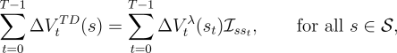
(7.8)

where is an identity indicator function, equal to if and equal to 0 otherwise.

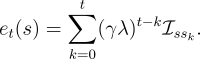
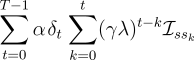
First note that an accumulating eligibility trace can be written explicitly (nonrecursively) as

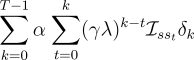
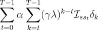
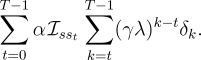
Thus, the left-hand side of (7.8) can be written

			(7.9)
			(7.10)
			(7.11)
			(7.12)

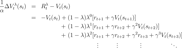
Now we turn to the right-hand side of (7.8). Consider an individual update of the $\lambda$-return algorithm:

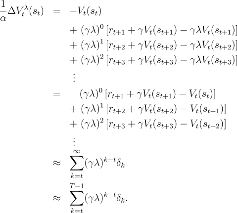
Examine the first column inside the brackets--all the 's with their weighting factors of times powers of $\lambda$. It turns out that all the weighting factors sum to 1. Thus we can pull out the first column and get an unweighted term of . A similar trick pulls out the second column in brackets, starting from the second row, which sums to . Repeating this for each column, we get

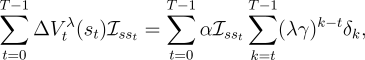
The approximation above is exact in the case of off-line updating, in which case is the same for all . The last step is exact (not an approximation) because all the terms omitted are due to fictitious steps "after" the terminal state has been entered. All these steps have zero rewards and zero values; thus all their 's are zero as well. Thus, we have shown that in the off-line case the right-hand side of (7.8) can be written

which is the same as (7.9). This proves (7.8).

In the case of on-line updating, the approximation made above will be close as long as $\alpha$ is small and thus changes little during an episode. Even in the on-line case we can expect the updates of TD($\lambda$) and of the $\lambda$-return algorithm to be similar.

For the moment let us assume that the increments are small enough during an episode that on-line TD($\lambda$) gives essentially the same update over the course of an episode as does the $\lambda$-return algorithm. There still remain interesting questions about what happens during an episode. Consider the updating of the value of state in midepisode, at time . Under on-line TD($\lambda$), the effect at is just as if we had done a $\lambda$-return update treating the last observed state as the terminal state of the episode with a nonzero terminal value equal to its current estimated value. This relationship is maintained from step to step as each new state is observed.

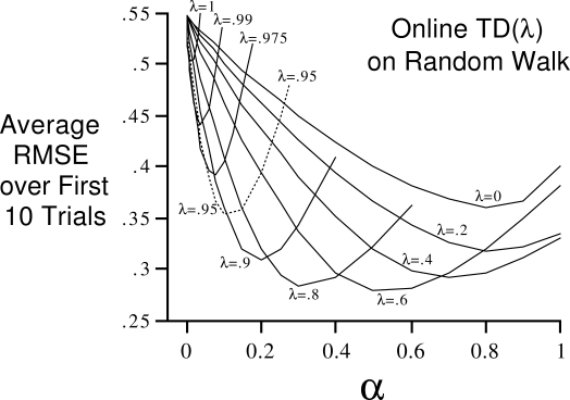
Example 7.3: Random Walk with TD($\lambda$)   Because off-line TD($\lambda$) is equivalent to the $\lambda$-return algorithm, we already have the results for off-line TD($\lambda$) on the 19-state random walk task; they are shown in Figure  7.6. The comparable results for on-line TD($\lambda$) are shown in Figure  7.9. Note that the on-line algorithm works better over a broader range of parameters. This is often found to be the case for on-line methods.

Figure 7.9: Performance of on-line TD($\lambda$) on the 19-state random walk task.

 

Exercise 7.5   Although TD($\lambda$) only approximates the $\lambda$-return algorithm when done online, perhaps there's a slightly different TD method that would maintain the equivalence even in the on-line case. One idea is to define the TD error instead as and the -step return as . Show that in this case the modified TD($\lambda$) algorithm would then achieve exactly

even in the case of on-line updating with large . In what ways might this modified TD($\lambda$) be better or worse than the conventional one described in the text? Describe an experiment to assess the relative merits of the two algorithms.