We begin by considering Monte Carlo methods for learning the state-value function for a given policy. Recall that the value of a state is the expected return--expected cumulative future discounted reward--starting from that state. An obvious way to estimate it from experience, then, is simply to average the returns observed after visits to that state. As more returns are observed, the average should converge to the expected value. This idea underlies all Monte Carlo methods.
In particular, suppose we wish to estimate ![]() , the value of a state
, the value of a state ![]() under policy
under policy ![]() , given a set of episodes obtained by following
, given a set of episodes obtained by following ![]() and
passing through
and
passing through ![]() . Each occurrence of state
. Each occurrence of state ![]() in an episode is
called a visit to
in an episode is
called a visit to ![]() . The every-visit MC
method estimates
. The every-visit MC
method estimates ![]() as the average of the returns following all the
visits to
as the average of the returns following all the
visits to ![]() in a set of episodes. Within a given episode, the first time
in a set of episodes. Within a given episode, the first time ![]() is visited is called the first visit to
is visited is called the first visit to ![]() . The first-visit MC
method averages just the returns following first visits to
. The first-visit MC
method averages just the returns following first visits to ![]() . These two
Monte Carlo methods are very similar but have slightly different theoretical
properties. First-visit MC has been most widely studied, dating back to the
1940s, and is the one we focus on in this chapter. We reconsider every-visit MC
in Chapter
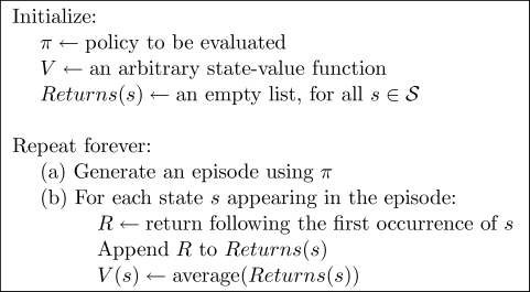
7. First-visit MC is shown in procedural form in
Figure
5.1.
. These two
Monte Carlo methods are very similar but have slightly different theoretical
properties. First-visit MC has been most widely studied, dating back to the
1940s, and is the one we focus on in this chapter. We reconsider every-visit MC
in Chapter
7. First-visit MC is shown in procedural form in
Figure
5.1.
Both first-visit MC and every-visit MC converge to ![]() as the number of
visits (or first visits) to
as the number of
visits (or first visits) to ![]() goes to infinity. This is easy to see for the
case of first-visit MC. In this case each return is an independent,
identically distributed estimate of
goes to infinity. This is easy to see for the
case of first-visit MC. In this case each return is an independent,
identically distributed estimate of
![]() . By the law of large numbers the sequence of averages
of these estimates converges to their expected value.
Each average is itself an unbiased estimate, and the standard deviation of its
error falls as
. By the law of large numbers the sequence of averages
of these estimates converges to their expected value.
Each average is itself an unbiased estimate, and the standard deviation of its
error falls as
![]() , where
, where ![]() is the number of returns averaged.
Every-visit MC is less straightforward, but its estimates also converge
asymptotically to
is the number of returns averaged.
Every-visit MC is less straightforward, but its estimates also converge
asymptotically to ![]() (Singh and Sutton,
1996).
(Singh and Sutton,
1996).
The use of Monte Carlo methods is best illustrated through an example.
Example 5.1 Blackjack is a popular casino card game. The object is to obtain cards the sum of whose numerical values is as great as possible without exceeding 21. All face cards count as 10, and the ace can count either as 1 or as 11. We consider the version in which each player competes independently against the dealer. The game begins with two cards dealt to both dealer and player. One of the dealer's cards is faceup and the other is facedown. If the player has 21 immediately (an ace and a 10-card), it is called a natural. He then wins unless the dealer also has a natural, in which case the game is a draw. If the player does not have a natural, then he can request additional cards, one by one (hits), until he either stops (sticks) or exceeds 21 (goes bust). If he goes bust, he loses; if he sticks, then it becomes the dealer's turn. The dealer hits or sticks according to a fixed strategy without choice: he sticks on any sum of 17 or greater, and hits otherwise. If the dealer goes bust, then the player wins; otherwise, the outcome--win, lose, or draw--is determined by whose final sum is closer to 21.
Playing blackjack is naturally formulated as an episodic finite MDP. Each
game of blackjack is an episode. Rewards of ![]() ,
, ![]() , and
, and ![]() are given for
winning, losing, and drawing, respectively. All rewards within a game are zero,
and we do not discount (
are given for
winning, losing, and drawing, respectively. All rewards within a game are zero,
and we do not discount (![]() ); therefore these terminal rewards are
also the returns. The player's actions are to hit or to stick.
The states depend on the player's cards and the dealer's showing card. We
assume that cards are dealt from an infinite deck (i.e., with replacement) so
that there is no advantage to keeping track of the cards already dealt. If the
player holds an ace that he could count as 11 without going bust, then the ace
is said to be usable. In this case it is always counted as 11 because
counting it as 1 would make the sum 11 or less, in which case
there is no decision to be made because, obviously, the player should always
hit. Thus, the player makes decisions on the basis of three variables: his
current sum (12-21), the dealer's one showing card (ace-10), and whether or
not he holds a usable ace. This makes for a total of 200 states.
); therefore these terminal rewards are
also the returns. The player's actions are to hit or to stick.
The states depend on the player's cards and the dealer's showing card. We
assume that cards are dealt from an infinite deck (i.e., with replacement) so
that there is no advantage to keeping track of the cards already dealt. If the
player holds an ace that he could count as 11 without going bust, then the ace
is said to be usable. In this case it is always counted as 11 because
counting it as 1 would make the sum 11 or less, in which case
there is no decision to be made because, obviously, the player should always
hit. Thus, the player makes decisions on the basis of three variables: his
current sum (12-21), the dealer's one showing card (ace-10), and whether or
not he holds a usable ace. This makes for a total of 200 states.
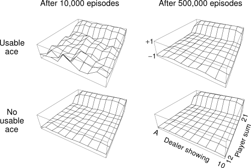
Consider the policy that sticks if the player's sum is 20 or 21, and otherwise hits. To find the state-value function for this policy by a Monte Carlo approach, one simulates many blackjack games using the policy and averages the returns following each state. Note that in this task the same state never recurs within one episode, so there is no difference between first-visit and every-visit MC methods. In this way, we obtained the estimates of the state-value function shown in Figure 5.2. The estimates for states with a usable ace are less certain and less regular because these states are less common. In any event, after 500,000 games the value function is very well approximated.
|
Although we have complete knowledge of the environment in this task, it would
not be easy to apply DP policy evaluation to compute the value function.
DP methods require the distribution of next events--in particular, they
require the quantities ![]() and
and ![]() --and it is not easy to
determine these for blackjack. For example, suppose the player's sum is 14
and he chooses to stick. What is his expected reward as a function of the
dealer's showing card? All of these expected rewards and transition
probabilities must be computed before DP can be applied, and such
computations are often complex and error-prone. In contrast, generating the
sample games required by Monte Carlo methods is easy. This is the case
surprisingly often; the ability of Monte Carlo methods to work with sample
episodes alone can be a significant advantage even when one has complete
knowledge of the environment's dynamics.
--and it is not easy to
determine these for blackjack. For example, suppose the player's sum is 14
and he chooses to stick. What is his expected reward as a function of the
dealer's showing card? All of these expected rewards and transition
probabilities must be computed before DP can be applied, and such
computations are often complex and error-prone. In contrast, generating the
sample games required by Monte Carlo methods is easy. This is the case
surprisingly often; the ability of Monte Carlo methods to work with sample
episodes alone can be a significant advantage even when one has complete
knowledge of the environment's dynamics.

Can we generalize the idea of backup diagrams to Monte Carlo
algorithms? The general idea of a backup diagram is to show at the top the
root node to be updated and to show below all the transitions and leaf nodes
whose rewards and estimated values contribute to the update. For Monte Carlo
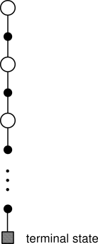
estimation of ![]() , the root is a state node, and below is
the entire sequence of transitions along a particular episode, ending at the
terminal state, as in Figure
5.3. Whereas the DP diagram
(Figure 3.4a) shows all possible transitions, the Monte Carlo diagram
shows only those sampled on the one episode. Whereas the DP diagram includes
only one-step transitions, the Monte Carlo diagram goes all the way to the end
of the episode. These differences in the diagrams accurately reflect the
fundamental differences between the algorithms.
, the root is a state node, and below is
the entire sequence of transitions along a particular episode, ending at the
terminal state, as in Figure
5.3. Whereas the DP diagram
(Figure 3.4a) shows all possible transitions, the Monte Carlo diagram
shows only those sampled on the one episode. Whereas the DP diagram includes
only one-step transitions, the Monte Carlo diagram goes all the way to the end
of the episode. These differences in the diagrams accurately reflect the
fundamental differences between the algorithms.
An important fact about Monte Carlo methods is that the estimates for each state are independent. The estimate for one state does not build upon the estimate of any other state, as is the case in DP. In other words, Monte Carlo methods do not "bootstrap" as we described it in the previous chapter.
In particular, note that the computational expense of estimating the value of a single state is independent of the number of states. This can make Monte Carlo methods particularly attractive when one requires the value of only a subset of the states. One can generate many sample episodes starting from these states, averaging returns only from of these states ignoring all others. This is a third advantage Monte Carlo methods can have over DP methods (after the ability to learn from actual experience and from simulated experience).
Example 5.2: Soap Bubble Suppose a wire frame forming a closed loop is dunked in soapy water to form a soap surface or bubble conforming at its edges to the wire frame. If the geometry of the wire frame is irregular but known, how can you compute the shape of the surface? The shape has the property that the total force on each point exerted by neighboring points is zero (or else the shape would change). This means that the surface's height at any point is the average of its heights at points in a small circle around that point. In addition, the surface must meet at its boundaries with the wire frame. The usual approach to problems of this kind is to put a grid over the area covered by the surface and solve for its height at the grid points by an iterative computation. Grid points at the boundary are forced to the wire frame, and all others are adjusted toward the average of the heights of their four nearest neighbors. This process then iterates, much like DP's iterative policy evaluation, and ultimately converges to a close approximation to the desired surface.
This is similar to the kind of problem for which Monte Carlo methods were originally designed. Instead of the iterative computation described above, imagine standing on the surface and taking a random walk, stepping randomly from grid point to neighboring grid point, with equal probability, until you reach the boundary. It turns out that the expected value of the height at the boundary is a close approximation to the height of the desired surface at the starting point (in fact, is is exactly the value computed by the iterative method described above). Thus, one can closely approximate the height of the surface at a point by simply averaging the boundary heights of many walks started at the point. If one is interested in only the value at one point, or any fixed small set of points, then this Monte Carlo method can be far more efficient than the iterative method based on local consistency.
Exercise 5.1 Consider the diagrams on the right in Figure 5.2. Why does the value function jump up for the last two rows in the rear? Why does it drop off for the whole last row on the left? Why are the frontmost values higher in the upper diagrams than in the lower?