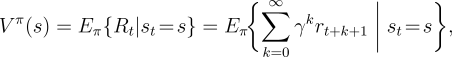
Almost all reinforcement learning algorithms are based on estimating value functions--functions of states (or of state-action pairs) that estimate how good it is for the agent to be in a given state (or how good it is to perform a given action in a given state). The notion of "how good" here is defined in terms of future rewards that can be expected, or, to be precise, in terms of expected return. Of course the rewards the agent can expect to receive in the future depend on what actions it will take. Accordingly, value functions are defined with respect to particular policies.
Recall that a policy, ![]() , is a mapping from each state,
, is a mapping from each state, ![]() , and action,
, and action, ![]() , to the probability
, to the probability ![]() of taking action
of taking action
![]() when in state
when in state ![]() . Informally, the value of a state
. Informally, the value of a state ![]() under a
policy
under a
policy
![]() , denoted
, denoted ![]() , is the expected return when starting in
, is the expected return when starting in ![]() and
following
and
following ![]() thereafter. For MDPs, we can define
thereafter. For MDPs, we can define ![]() formally as
formally as
Similarly, we define the value of taking action ![]() in
state
in
state ![]() under a policy
under a policy ![]() , denoted
, denoted ![]() , as the expected
return starting from
, as the expected
return starting from ![]() , taking the action
, taking the action ![]() , and thereafter following
policy
, and thereafter following
policy ![]() :
:
The value functions ![]() and
and ![]() can be estimated from
experience. For example, if an agent follows policy
can be estimated from
experience. For example, if an agent follows policy
![]() and maintains an average, for each state encountered, of the actual returns
that have followed that state, then the average will converge to
the state's value,
and maintains an average, for each state encountered, of the actual returns
that have followed that state, then the average will converge to
the state's value, ![]() , as the number of times that state is
encountered approaches infinity. If separate averages are kept for each action taken
in a state, then these averages will similarly converge to the action values,
, as the number of times that state is
encountered approaches infinity. If separate averages are kept for each action taken
in a state, then these averages will similarly converge to the action values,
![]() . We call estimation methods of this kind Monte Carlo
methods because they involve averaging over many random samples
of actual returns. These kinds of methods are presented in Chapter 5. Of
course, if there are very many states, then it may not be practical to keep
separate averages for each state individually. Instead, the agent would have to
maintain
. We call estimation methods of this kind Monte Carlo
methods because they involve averaging over many random samples
of actual returns. These kinds of methods are presented in Chapter 5. Of
course, if there are very many states, then it may not be practical to keep
separate averages for each state individually. Instead, the agent would have to
maintain
![]() and
and ![]() as parameterized functions and adjust the parameters to
better match the observed returns. This can also produce accurate estimates,
although much depends on the nature of the parameterized function approximator
(Chapter 8).
as parameterized functions and adjust the parameters to
better match the observed returns. This can also produce accurate estimates,
although much depends on the nature of the parameterized function approximator
(Chapter 8).
A fundamental property of value functions used throughout reinforcement learning
and dynamic programming is that they satisfy
particular recursive relationships. For any
policy ![]() and any state
and any state
![]() , the following consistency condition holds between the value of
, the following consistency condition holds between the value of ![]() and the value
of its possible successor states:
and the value
of its possible successor states:
The value function ![]() is the unique solution to its Bellman
equation. We show in subsequent chapters
how this Bellman equation forms the basis of a number of ways to compute,
approximate, and learn
is the unique solution to its Bellman
equation. We show in subsequent chapters
how this Bellman equation forms the basis of a number of ways to compute,
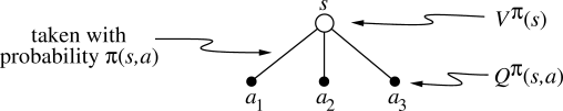
approximate, and learn ![]() . We call diagrams like those shown in
Figure
3.4 backup diagrams because they diagram
relationships that form the basis of the update or backup operations that are
at the heart of reinforcement learning methods. These operations transfer value
information back to a state (or a state-action pair) from its successor states
(or state-action pairs). We use backup diagrams throughout the book to provide
graphical summaries of the algorithms we discuss. (Note that unlike transition
graphs, the state nodes of backup diagrams do not necessarily represent distinct
states; for example, a state might be its own successor. We also omit explicit
arrowheads because time always flows downward in a backup diagram.)
. We call diagrams like those shown in
Figure
3.4 backup diagrams because they diagram
relationships that form the basis of the update or backup operations that are
at the heart of reinforcement learning methods. These operations transfer value
information back to a state (or a state-action pair) from its successor states
(or state-action pairs). We use backup diagrams throughout the book to provide
graphical summaries of the algorithms we discuss. (Note that unlike transition
graphs, the state nodes of backup diagrams do not necessarily represent distinct
states; for example, a state might be its own successor. We also omit explicit
arrowheads because time always flows downward in a backup diagram.)
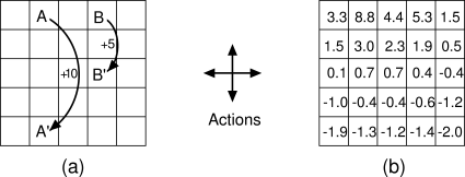
Example 3.8: Gridworld Figure 3.5a uses a rectangular grid to illustrate value functions for a simple finite MDP. The cells of the grid correspond to the states of the environment. At each cell, four actions are possible: north, south, east, and west, which deterministically cause the agent to move one cell in the respective direction on the grid. Actions that would take the agent off the grid leave its location unchanged, but also result in a reward of
|
Suppose the agent selects all four actions with equal probability in all
states. Figure
3.5b shows the value function,
![]() , for this policy, for the discounted reward case with
, for this policy, for the discounted reward case with ![]() . This
value function was computed by solving the system of equations
(3.10). Notice the negative values near the lower
edge; these are the result of the high probability of hitting the edge
of the grid there under the random policy. State A
is the best state to be in under this policy, but its expected return is less
than 10, its immediate reward, because from A the agent is taken to
. This
value function was computed by solving the system of equations
(3.10). Notice the negative values near the lower
edge; these are the result of the high probability of hitting the edge
of the grid there under the random policy. State A
is the best state to be in under this policy, but its expected return is less
than 10, its immediate reward, because from A the agent is taken to
![]() , from which it is likely to run into the edge of the grid. State B, on
the other hand, is valued more than 5, its immediate reward, because from B the agent
is taken to
, from which it is likely to run into the edge of the grid. State B, on
the other hand, is valued more than 5, its immediate reward, because from B the agent
is taken to ![]() , which has a positive value. From
, which has a positive value. From ![]() the expected penalty
(negative reward) for possibly running into an edge is more than compensated for by
the expected gain for possibly stumbling onto A or B.
the expected penalty
(negative reward) for possibly running into an edge is more than compensated for by
the expected gain for possibly stumbling onto A or B.

|
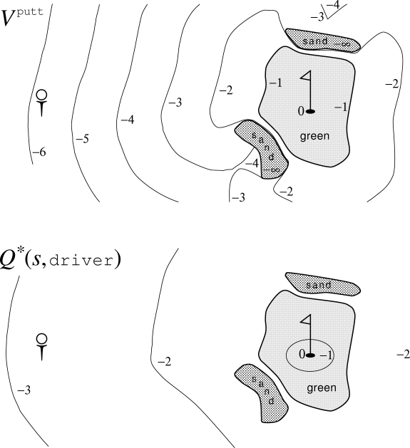
Example 3.9: Golf To formulate playing a hole of golf as a reinforcement learning task, we count a penalty (negative reward) of
Exercise 3.8 What is the Bellman equation for action values, that is, for
Exercise 3.9 The Bellman equation (3.10) must hold for each state for the value function
Exercise 3.10 In the gridworld example, rewards are positive for goals, negative for running into the edge of the world, and zero the rest of the time. Are the signs of these rewards important, or only the intervals between them? Prove, using (3.2), that adding a constant
Exercise 3.11 Now consider adding a constant
Exercise 3.12 The value of a state depends on the the values of the actions possible in that state and on how likely each action is to be taken under the current policy. We can think of this in terms of a small backup diagram rooted at the state and considering each possible action:
|
Exercise 3.13 The value of an action,

|