2.6 Tracking a Nonstationary Problem

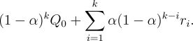
The averaging methods discussed so far are appropriate in a stationary environment, but not if the bandit is changing over time. As noted earlier, we often encounter reinforcement learning problems that are effectively nonstationary. In such cases it makes sense to weight recent rewards more heavily than long-past ones. One of the most popular ways of doing this is to use a constant step-size parameter. For example, the incremental update rule (2.4) for updating an average of the past rewards is modified to be

(2.6)

where the step-size parameter, , , is constant. This results in being a weighted average of past rewards and the initial estimate :

			(2.7)

We call this a weighted average because the sum of the weights is , as you can check yourself. Note that the weight, , given to the reward depends on how many rewards ago, , it was observed. The quantity is less than , and thus the weight given to decreases as the number of intervening rewards increases. In fact, the weight decays exponentially according to the exponent on . Accordingly, this is sometimes called an exponential, recency-weighted average.

Sometimes it is convenient to vary the step-size parameter from step to step. Let denote the step-size parameter used to process the reward received after the th selection of action . As we have noted, the choice results in the sample-average method, which is guaranteed to converge to the true action values by the law of large numbers. But of course convergence is not guaranteed for all choices of the sequence . 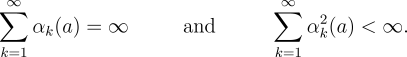A well-known result in stochastic approximation theory gives us the conditions required to assure convergence with probability 1:

(2.8)

The first condition is required to guarantee that the steps are large enough to eventually overcome any initial conditions or random fluctuations. The second condition guarantees that eventually the steps become small enough to assure convergence.

Note that both convergence conditions are met for the sample-average case, , but not for the case of constant step-size parameter, . In the latter case, the second condition is not met, indicating that the estimates never completely converge but continue to vary in response to the most recently received rewards. As we mentioned above, this is actually desirable in a nonstationary environment, and problems that are effectively nonstationary are the norm in reinforcement learning. In addition, sequences of step-size parameters that meet the conditions (2.8) often converge very slowly or need considerable tuning in order to obtain a satisfactory convergence rate. Although sequences of step-size parameters that meet these convergence conditions are often used in theoretical work, they are seldom used in applications and empirical research.

Exercise 2.6   If the step-size parameters, , are not constant, then the estimate is a weighted average of previously received rewards with a weighting different from that given by (2.7). What is the weighting on each prior reward for the general case?

Exercise 2.7 (programming)   Design and conduct an experiment to demonstrate the difficulties that sample-average methods have for nonstationary problems. Use a modified version of the 10-armed testbed in which all the start out equal and then take independent random walks. Prepare plots like Figure  2.1 for an action-value method using sample averages, incrementally computed by , and another action-value method using a a constant step-size parameter, . Use and, if necessary, runs longer than 1000 plays.