Waiting for an elevator is a situation with which we are all familiar. We press a button and then wait for an elevator to arrive traveling in the right direction. We may have to wait a long time if there are too many passengers or not enough elevators. Just how long we wait depends on the dispatching strategy the elevators use to decide where to go. For example, if passengers on several floors have requested pickups, which should be served first? If there are no pickup requests, how should the elevators distribute themselves to await the next request? Elevator dispatching is a good example of a stochastic optimal control problem of economic importance that is too large to solve by classical techniques such as dynamic programming.
Crites and Barto (1996; Crites, 1996)
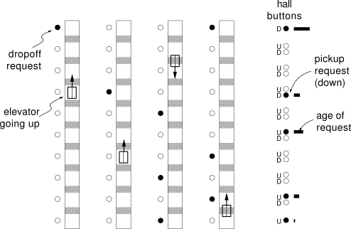
studied the application of reinforcement learning techniques to the
four-elevator, ten-floor system shown in Figure
11.8. Along the
right-hand side are pickup requests
and an indication of how long each has been waiting. Each elevator has a
position, direction, and speed, plus a set of buttons to indicate where
passengers want to get off. Roughly quantizing the continuous variables, Crites
and Barto estimated that the system has over ![]() states. This large
state set rules out classical dynamic programming methods such as value
iteration. Even if one state could be backed up every microsecond it would
still require over 1000 years to complete just one sweep through the state space.
states. This large
state set rules out classical dynamic programming methods such as value
iteration. Even if one state could be backed up every microsecond it would
still require over 1000 years to complete just one sweep through the state space.
In practice, modern elevator dispatchers are designed heuristically and evaluated on simulated buildings. The simulators are quite sophisticated and detailed. The physics of each elevator car is modeled in continuous time with continuous state variables. Passenger arrivals are modeled as discrete, stochastic events, with arrival rates varying frequently over the course of a simulated day. Not surprisingly, the times of greatest traffic and greatest challenge to the dispatching algorithm are the morning and evening rush hours. Dispatchers are generally designed primarily for these difficult periods.
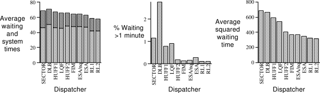
The performance of elevator dispatchers is measured in several different ways, all with respect to an average passenger entering the system. The average waiting time is how long the passenger waits before getting on an elevator, and the average system time is how long the passenger waits before being dropped off at the destination floor. Another frequently encountered statistic is the percentage of passengers whose waiting time exceeds 60 seconds. The objective that Crites and Barto focused on is the average squared waiting time. This objective is commonly used because it tends to keep the waiting times low while also encouraging fairness in serving all the passengers.
Crites and Barto applied a version of one-step Q-learning augmented in several ways to take advantage of special features of the problem. The most important of these concerned the formulation of the actions. First, each elevator made its own decisions independently of the others. Second, a number of constraints were placed on the decisions. An elevator carrying passengers could not pass by a floor if any of its passengers wanted to get off there, nor could it reverse direction until all of its passengers wanting to go in its current direction had reached their floors. In addition, a car was not allowed to stop at a floor unless someone wanted to get on or off there, and it could not stop to pick up passengers at a floor if another elevator was already stopped there. Finally, given a choice between moving up or down, the elevator was constrained always to move up (otherwise evening rush hour traffic would tend to push all the elevators down to the lobby). These last three constraints were explicitly included to provide some prior knowledge and make the problem easier. The net result of all these constraints was that each elevator had to make few and simple decisions. The only decision that had to be made was whether or not to stop at a floor that was being approached and that had passengers waiting to be picked up. At all other times, no choices needed to be made.
That each elevator made choices only infrequently permitted
a second simplification of the problem. As far as the learning agent was
concerned, the system made discrete jumps from one time at which
it had to make a decision to the next. When a continuous-time decision problem is
treated as a discrete-time system in this way it is known as a semi-Markov
decision process. To a large extent, such processes can be treated just like any
other Markov decision process by taking the reward on each discrete transition as
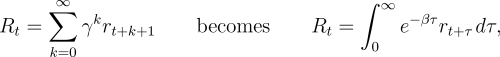
the integral of the reward over the corresponding continuous-time interval. The
notion of return generalizes naturally from a discounted sum of future rewards to a
discounted integral of future rewards:
|
The basic idea of the extension of Q-learning to semi-Markov
decision problems can now be explained. Suppose the system is in state ![]() and
takes action
and
takes action ![]() at time
at time ![]() , and then the next decision is required at time
, and then the next decision is required at time
![]() in state
in state ![]() . After this discrete-event transition, the
semi-Markov Q-learning backup for a tabular action-value function,
. After this discrete-event transition, the
semi-Markov Q-learning backup for a tabular action-value function, ![]() , would
be:
, would
be:

|
One complication is that the reward as defined--the negative sum of the squared waiting times--is not something that would normally be known while an actual elevator was running. This is because in a real elevator system one does not know how many people are waiting at a floor, only how long it has been since the button requesting a pickup on that floor was pressed. Of course this information is known in a simulator, and Crites and Barto used it to obtain their best results. They also experimented with another technique that used only information that would be known in an on-line learning situation with a real set of elevators. In this case one can use how long since each button has been pushed together with an estimate of the arrival rate to compute an expected summed squared waiting time for each floor. Using this in the reward measure proved nearly as effective as using the actual summed squared waiting time.
For function approximation, a nonlinear neural network trained by backpropagation was used to represent the action-value function. Crites and Barto experimented with a wide variety of ways of representing states to the network. After much exploration, their best results were obtained using networks with 47 input units, 20 hidden units, and two output units, one for each action. The way the state was encoded by the input units was found to be critical to the effectiveness of the learning. The 47 input units were as follows:
Two architectures were used. In RL1, each elevator was given its own action-value function and its own neural network. In RL2, there was only one network and one action-value function, with the experiences of all four elevators contributing to learning in the one network. In both cases, each elevator made its decisions independently of the other elevators, but shared a single reward signal with them. This introduced additional stochasticity as far as each elevator was concerned because its reward depended in part on the actions of the other elevators, which it could not control. In the architecture in which each elevator had its own action-value function, it was possible for different elevators to learn different specialized strategies (although in fact they tended to learn the same strategy). On the other hand, the architecture with a common action-value function could learn faster because it learned simultaneously from the experiences of all elevators. Training time was an issue here, even though the system was trained in simulation. The reinforcement learning methods were trained for about four days of computer time on a 100 mips processor (corresponding to about 60,000 hours of simulated time). While this is a considerable amount of computation, it is negligible compared with what would be required by any conventional dynamic programming algorithm.
The networks were trained by simulating a great many evening rush hours while making dispatching decisions using the developing, learned action-value functions. Crites and Barto used the Gibbs softmax procedure to select actions as described in Section 2.3, reducing the "temperature" gradually over training. A temperature of zero was used during test runs on which the performance of the learned dispatchers was assessed.
Figure 11.9 shows the performance of several dispatchers during a simulated evening rush hour, what researchers call down-peak traffic. The dispatchers include methods similar to those commonly used in the industry, a variety of heuristic methods, sophisticated research algorithms that repeatedly run complex optimization algorithms on-line (Bao et al., 1994), and dispatchers learned by using the two reinforcement learning architectures. By all of the performance measures, the reinforcement learning dispatchers compare favorably with the others. Although the optimal policy for this problem is unknown, and the state of the art is difficult to pin down because details of commercial dispatching strategies are proprietary, these learned dispatchers appeared to perform very well.