One of the most impressive applications of reinforcement learning to date
is that by Gerry Tesauro to the game of backgammon (Tesauro, 1992, 1994,
1995). Tesauro's program,
TD-Gammon, required little backgammon knowledge, yet learned to play
extremely well, near the level of the world's strongest grandmasters. The
learning algorithm in TD-Gammon was a straightforward combination of the
TD(![]() ) algorithm and nonlinear function approximation using a
multilayer neural network trained by backpropagating TD errors.
) algorithm and nonlinear function approximation using a
multilayer neural network trained by backpropagating TD errors.
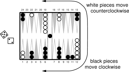
Backgammon is a major game in the sense that it is played throughout the world, with numerous tournaments and regular world championship matches. It is in part a game of chance, and it is a popular vehicle for waging significant sums of money. There are probably more professional backgammon players than there are professional chess players. The game is played with 15 white and 15 black pieces on a board of 24 locations, called points. Figure 11.1 shows a typical position early in the game, seen from the perspective of the white player.
In this figure, white has just rolled the dice and obtained a 5 and a 2. This means that he can move one of his pieces 5 steps and one (possibly the same piece) 2 steps. For example, he could move two pieces from the 12 point, one to the 17 point, and one to the 14 point. White's objective is to advance all of his pieces into the last quadrant (points 19-24) and then off the board. The first player to remove all his pieces wins. One complication is that the pieces interact as they pass each other going in different directions. For example, if it were black's move in Figure 11.1, he could use the dice roll of 2 to move a piece from the 24 point to the 22 point, "hitting" the white piece there. Pieces that have been hit are placed on the "bar" in the middle of the board (where we already see one previously hit black piece), from whence they reenter the race from the start. However, if there are two pieces on a point, then the opponent cannot move to that point; the pieces are protected from being hit. Thus, white cannot use his 5-2 dice roll to move either of his pieces on the 1 point, because their possible resulting points are occupied by groups of black pieces. Forming contiguous blocks of occupied points to block the opponent is one of the elementary strategies of the game.
Backgammon involves several further complications, but the above description gives the basic idea. With 30 pieces and 24 possible locations (26, counting the bar and off-the-board) it should be clear that the number of possible backgammon positions is enormous, far more than the number of memory elements one could have in any physically realizable computer. The number of moves possible from each position is also large. For a typical dice roll there might be 20 different ways of playing. In considering future moves, such as the response of the opponent, one must consider the possible dice rolls as well. The result is that the game tree has an effective branching factor of about 400. This is far too large to permit effective use of the conventional heuristic search methods that have proved so effective in games like chess and checkers.
On the other hand, the game is a good match to the capabilities of TD learning methods. Although the game is highly stochastic, a complete description of the game's state is available at all times. The game evolves over a sequence of moves and positions until finally ending in a win for one player or the other, ending the game. The outcome can be interpreted as a final reward to be predicted. On the other hand, the theoretical results we have described so far cannot be usefully applied to this task. The number of states is so large that a lookup table cannot be used, and the opponent is a source of uncertainty and time variation.
TD-Gammon used a nonlinear form of TD(![]() ).
The estimated value,
).
The estimated value, ![]() , of any state (board position)
, of any state (board position) ![]() was meant to estimate the probability of winning starting from state
was meant to estimate the probability of winning starting from state ![]() .
To achieve this, rewards were defined as zero for all time steps except those on
which the game is won. To implement the value function, TD-Gammon used a
standard multilayer neural network, much as shown in Figure
11.2.
(The real network had two additional units in its final
layer to estimate the probability of each player's winning in a special way
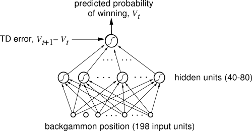
called a "gammon" or "backgammon.") The network consisted of a layer of input
units, a layer of hidden units, and a final output unit. The input to the
network was a representation of a backgammon position, and
the output was an estimate of the value of that position.
.
To achieve this, rewards were defined as zero for all time steps except those on
which the game is won. To implement the value function, TD-Gammon used a
standard multilayer neural network, much as shown in Figure
11.2.
(The real network had two additional units in its final
layer to estimate the probability of each player's winning in a special way
called a "gammon" or "backgammon.") The network consisted of a layer of input
units, a layer of hidden units, and a final output unit. The input to the
network was a representation of a backgammon position, and
the output was an estimate of the value of that position.
In the first version of TD-Gammon, TD-Gammon 0.0, backgammon positions were
represented to the network in a relatively direct way that involved little
backgammon knowledge. It did, however, involve substantial knowledge of how
neural networks work and how information is best presented to them. It is
instructive to note the exact representation Tesauro chose.
There were a total of
198 input units to the network. For each point on the backgammon board, four units
indicated the number of white pieces on the point. If there were no white pieces,
then all four units took on the value zero. If there was one piece, then the first
unit took on the value 1. If there were two pieces, then both the first and the
second unit were 1. If there were three or more pieces on the point, then all of
the first three units were 1. If there were more than three pieces, the fourth
unit also came on, to a degree indicating the number of additional pieces beyond
three. Letting ![]() denote the total number of pieces on the point, if
denote the total number of pieces on the point, if ![]() ,
then the fourth unit took on the value
,
then the fourth unit took on the value ![]() . With four units for white and
four for black at each of the 24 points, that made a total of 192 units. Two
additional units encoded the number of white and black pieces on the bar (each took the
value
. With four units for white and
four for black at each of the 24 points, that made a total of 192 units. Two
additional units encoded the number of white and black pieces on the bar (each took the
value ![]() , where
, where ![]() is the number of pieces on the bar), and two more encoded the
number of black and white pieces already successfully removed from the board (these
took the value
is the number of pieces on the bar), and two more encoded the
number of black and white pieces already successfully removed from the board (these
took the value ![]() , where
, where ![]() is the number of pieces already borne off).
Finally, two units indicated in a binary fashion whether it was white's or black's turn
to move. The general logic behind these choices should be clear. Basically, Tesauro
tried to represent the position in a straightforward way, making little attempt
to minimize the number of units. He provided one unit for each conceptually distinct
possibility that seemed likely to be relevant, and he scaled them to roughly the same
range, in this case between 0 and 1.
is the number of pieces already borne off).
Finally, two units indicated in a binary fashion whether it was white's or black's turn
to move. The general logic behind these choices should be clear. Basically, Tesauro
tried to represent the position in a straightforward way, making little attempt
to minimize the number of units. He provided one unit for each conceptually distinct
possibility that seemed likely to be relevant, and he scaled them to roughly the same
range, in this case between 0 and 1.
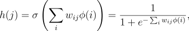
Given a representation of a backgammon position, the network computed its
estimated value in the standard way. Corresponding to each connection
from an input unit to a hidden unit was a real-valued weight. Signals from each
input unit were multiplied by their corresponding weights and summed at the hidden
unit. The output, ![]() , of hidden unit
, of hidden unit ![]() was a nonlinear sigmoid function
of the weighted sum:
was a nonlinear sigmoid function
of the weighted sum:
|
TD-Gammon used the
gradient-descent form of the TD(![]() ) algorithm described in Section 8.2, with the
gradients computed by the error backpropagation algorithm (Rumelhart, Hinton,
and Williams, 1986). Recall
that the general update rule for this case is
) algorithm described in Section 8.2, with the
gradients computed by the error backpropagation algorithm (Rumelhart, Hinton,
and Williams, 1986). Recall
that the general update rule for this case is
To apply the learning rule we need a source of backgammon games.
Tesauro obtained an unending sequence of games by playing his
learning backgammon player against itself. To choose its moves, TD-Gammon
considered each of the 20 or so ways it could play its dice roll and the
corresponding positions that would result. The resulting positions are afterstates as discussed in Section 6.8. The network was consulted
to estimate each of their values. The move was then selected that would lead
to the position with the highest estimated value. Continuing in this way, with
TD-Gammon making the moves for both sides, it was possible to easily generate large
numbers of backgammon games. Each game was treated as an episode, with the sequence
of positions acting as the states, ![]() . Tesauro applied the
nonlinear TD rule (11.1) fully incrementally, that is, after each
individual move.
. Tesauro applied the
nonlinear TD rule (11.1) fully incrementally, that is, after each
individual move.
The weights of the network were set initially to small random values. The initial evaluations were thus entirely arbitrary. Since the moves were selected on the basis of these evaluations, the initial moves were inevitably poor, and the initial games often lasted hundreds or thousands of moves before one side or the other won, almost by accident. After a few dozen games however, performance improved rapidly.
After playing about 300,000 games against itself, TD-Gammon 0.0 as described above learned to play approximately as well as the best previous backgammon computer programs. This was a striking result because all the previous high-performance computer programs had used extensive backgammon knowledge. For example, the reigning champion program at the time was, arguably, Neurogammon, another program written by Tesauro that used a neural network but not TD learning. Neurogammon's network was trained on a large training corpus of exemplary moves provided by backgammon experts, and, in addition, started with a set of features specially crafted for backgammon. Neurogammon was a highly tuned, highly effective backgammon program that decisively won the World Backgammon Olympiad in 1989. TD-Gammon 0.0, on the other hand, was constructed with essentially zero backgammon knowledge. That it was able to do as well as Neurogammon and all other approaches is striking testimony to the potential of self-play learning methods.
The tournament success of TD-Gammon 0.0 with zero backgammon knowledge suggested an obvious modification: add the specialized backgammon features but keep the self-play TD learning method. This produced TD-Gammon 1.0. TD-Gammon 1.0 was clearly substantially better than all previous backgammon programs and found serious competition only among human experts. Later versions of the program, TD-Gammon 2.0 (40 hidden units) and TD-Gammon 2.1 (80 hidden units), were augmented with a selective two-ply search procedure. To select moves, these programs looked ahead not just to the positions that would immediately result, but also to the opponent's possible dice rolls and moves. Assuming the opponent always took the move that appeared immediately best for him, the expected value of each candidate move was computed and the best was selected. To save computer time, the second ply of search was conducted only for candidate moves that were ranked highly after the first ply, about four or five moves on average. Two-ply search affected only the moves selected; the learning process proceeded exactly as before. The most recent version of the program, TD-Gammon 3.0, uses 160 hidden units and a selective three-ply search. TD-Gammon illustrates the combination of learned value functions and decide-time search as in heuristic search methods. In more recent work, Tesauro and Galperin (1997) have begun exploring trajectory sampling methods as an alternative to search.
Tesauro was able to play his programs in a significant number of games against world-class human players. A summary of the results is given in Table 11.1. Based on these results and analyses by backgammon grandmasters (Robertie, 1992; see Tesauro, 1995), TD-Gammon 3.0 appears to be at, or very near, the playing strength of the best human players in the world. It may already be the world champion. These programs have already changed the way the best human players play the game. For example, TD-Gammon learned to play certain opening positions differently than was the convention among the best human players. Based on TD-Gammon's success and further analysis, the best human players now play these positions as TD-Gammon does (Tesauro, 1995).