


To illustrate the general idea of reinforcement learning and contrast it with other approaches, we next consider a single example in more detail.
Consider the familiar child's game of Tic-Tac-Toe. Two players take turns playing on a three-by-three board. One player plays X s and the other Ø s until one player wins by placing three of his marks in a row, horizontally, vertically, or diagonally, as the `X ' player has in this game:

If the board fills up with neither player getting three in a row, the game is a draw. Because a skilled player can play so that he never loses, let us assume that we are playing against an imperfect player, one whose play is sometimes incorrect and allows us to win. For the moment, in fact, let us consider draws and losses to be equally bad for us. How might we construct a player that will find the imperfections in its opponent's play and learn to maximize its chances of winning?
Although this is a very simple problem, it cannot readily be solved in a satisfactory way by classical techniques. For example, the classical ``minimax" solution from game theory is not correct here because it assumes a particular way of playing by the opponent. For example, a minimax player would never reach a game state from which it could lose, even if in fact it always won from that state because of incorrect play by the opponent. Classical optimization methods for sequential decision problems, such as dynamic programming, can compute an optimal solution for any opponent, but require as input a complete specification of that opponent, including the probabilities with which the opponent makes each move in each board state. Let us assume that this information is not available a priori for this problem, as it is not for the vast majority of problems of practical interest. On the other hand, such information can be estimated from experience, in this case by playing many games against the opponent. About the best one can do on this problem is to first learn a model of the opponent's behavior, up to some level of confidence, and then apply dynamic programming to compute an optimal solution given the approximate opponent model. In the end, this is not that different from some of the reinforcement learning methods we examine later in this book.
An evolutionary approach to this problem would directly search the space of possible policies for one with a high probability of winning against the opponent. Here, a policy is a rule that tells the player what move to make for every state of the game---every possible configuration of X s and Ø s on the three-by-three board. For each policy considered, an estimate of its winning probability would be obtained by playing some number of games against the opponent. This evaluation would then direct which policy or policies were next considered. A typical evolutionary method would hillclimb in policy space, successively generating and evaluating policies in an attempt to obtain incremental improvements. Or, perhaps, a genetic-style algorithm could be used which would maintain and evaluate a population of policies. Literally hundreds of different optimization algorithms could be applied. By directly searching the policy space we mean that entire policies are proposed and compared on the basis of scalar evaluations.
Here is how the Tic-Tac-Toe problem would be approached using reinforcement learning and approximate value functions. First we set up a table of numbers, one for each possible state of the game. Each number will be the latest estimate of the probability of our winning from that state. We treat this estimate as the state's current value, and the whole table is the learned value function. State A has higher value than state B, or is considered ``better" than state B, if the current estimate of the probability of our winning from A is higher than it is from B. Assuming we always play X s, then for all states with three X s in a row the probability of winning is 1, because we have already won. Similarly, for all states with three Ø s in a row, or that are ``filled up", the correct probability is 0, as we cannot win from them. We set the initial values of all the other states, the nonterminals, to 0.5, representing an informed guess that we have a 50% chance of winning.
Now we play many games against the opponent. To select our moves we examine the states that would result from each of our possible moves (one for each blank space on the board) and look up their current values in the table. Most of the time we move greedily, selecting the move that leads to the state with greatest value, that is, with the highest estimated probability of winning. Occasionally, however, we select randomly from one of the other moves instead; these are called exploratory moves because they cause us to experience states that we might otherwise never see. A sequence of moves made and considered during a game can be diagrammed as in Figure 1.1.
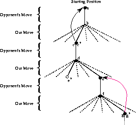
Figure 1.1: A sequence of Tic-Tac-Toe moves. The solid lines represent the moves
taken during a game; the dashed lines represent moves that we (our algorithm)
considered but did not make. Our second move was an exploratory
move, meaning that is was taken even though another sibling move,
that leading to  , was ranked higher. Exploratory moves do
not result in any learning, but each of our other moves do, causing
backups as suggested by the curved arrows and detailed in the text.
, was ranked higher. Exploratory moves do
not result in any learning, but each of our other moves do, causing
backups as suggested by the curved arrows and detailed in the text.
While we are playing, we change the values of the states in which we find
ourselves during the game. We attempt to make them more accurate estimates of the
probabilities of winning from those states. To do this, we ``back up"
the value of the state after each greedy move to the state
before the move, as suggested by the arrows in Figure 1.1.
More precisely, the current value of the earlier state is adjusted to be
closer to the value of the later state. This can be done by moving the
earlier state's value a fraction of the way toward the value of the later
state. If we let s denote the state before the greedy move, and  the
state after, then the update to the estimated value of s, denoted
the
state after, then the update to the estimated value of s, denoted  ,
can be written:
,
can be written:

where  is a small positive fraction called the step-size
parameter, which influences the rate of learning. This update rule is an
example of a temporal-difference learning method, so called because
it's changes are based on a difference,
is a small positive fraction called the step-size
parameter, which influences the rate of learning. This update rule is an
example of a temporal-difference learning method, so called because
it's changes are based on a difference, 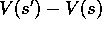 , between estimates at
two different times.
, between estimates at
two different times.
The method described above performs quite well on this task. For example, if the step-size parameter is reduced properly over time, this method converges, for any fixed opponent, to the true probabilities of winning from each state given optimal play by our player. Furthermore, the moves then taken (except on exploratory moves) are in fact the optimal moves against the opponent. In other words, the method converges to an optimal policy for playing the game. If the step-size parameter is not reduced all the way to zero over time, then this player also plays well against opponents that change their way of playing slowly over time.
This example illustrates the differences between evolutionary methods and methods that learn value functions. To evaluate a policy, an evolutionary method must hold it fixed and play many games against the opponent, or simulate many games using a model of the opponent. The frequency of wins gives an unbiased estimate of the probability of winning with that policy, and can be used to direct the next policy selection. But each policy change is made only after many games, and only the final outcome of each game is used: what happens during the games is ignored. For example, if the player wins, then all of its behavior in the game is given credit, independently of how specific moves might have been critical to the win. Credit is even given to moves that never occurred! Value function methods, in contrast, allow individual states to be evaluated. In the end, both evolutionary and value function methods search the space of policies, but learning a value function takes advantage of information available during the course of play.
This example is very simple, but it illustrates some of the key features of reinforcement learning methods. First, there is the emphasis on learning while interacting with an environment, in this case with an opponent player. Second, there is a clear goal, and correct behavior requires planning or foresight that takes into account delayed effects of one's choices. For example, the simple reinforcement learning player would learn to set up multi-move traps for a short-sighted opponent. It is a striking feature of the reinforcement learning solution that it can achieve the effects of planning and lookahead without using a model of the opponent and without carrying out an explicit search over possible sequences of future states and actions.
While this example illustrates some of the key features of reinforcement learning, it is so simple that it might give the impression that reinforcement learning is more limited than it really is. Although Tic-Tac-Toe is a two-person game, reinforcement learning also applies when there is no explicit external adversary, that is, in the case of a ``game against nature." \ Reinforcement learning is also not restricted to problems in which behavior breaks down into separate episodes, like the separate games of Tic-Tac-Toe, with reward only at the end of each episode. It is just as applicable when behavior continues indefinitely and when rewards of various magnitudes can be received at any time.
Tic-Tac-Toe has a relatively small, finite state set, whereas reinforcement
learning can be applied to very large, or even infinite, state sets. For
example, Gerry Tesauro (1992, 1995)
combined the algorithm described above with an artificial neural network to learn
to play the game of backgammon, which has approximately  states. Notice
that with this many states it is impossible to ever experience more than a small
fraction of them. Tesauro's program learned to play far better than any previous
program, and now plays at the level of the world's best human players (see
Chapter 11
). The neural network provides the program with the ability to
generalize from its experience, so that in new states it selects moves based on
information saved from similar states faced in the past, as determined by its
network. How well a reinforcement learning agent can work in problems with such
large state sets is intimately tied to how appropriately it can generalize from
past experience. It is in this role that we have the greatest need for supervised
learning methods with reinforcement learning. Neural networks are not the
only, or necessarily the best, way to do this.
states. Notice
that with this many states it is impossible to ever experience more than a small
fraction of them. Tesauro's program learned to play far better than any previous
program, and now plays at the level of the world's best human players (see
Chapter 11
). The neural network provides the program with the ability to
generalize from its experience, so that in new states it selects moves based on
information saved from similar states faced in the past, as determined by its
network. How well a reinforcement learning agent can work in problems with such
large state sets is intimately tied to how appropriately it can generalize from
past experience. It is in this role that we have the greatest need for supervised
learning methods with reinforcement learning. Neural networks are not the
only, or necessarily the best, way to do this.
In this Tic-Tac-Toe example, learning started with no prior knowledge beyond the rules of the game, but reinforcement learning by no means entails a tabula rasa view of learning and intelligence. On the contrary, prior information can be incorporated into reinforcement learning in a variety of ways that can be critical for efficient learning. We also had access to the true state in the Tic-Tac-Toe example, whereas reinforcement learning can also be applied when part of the state is hidden, or when different states appear to the learner to be the same. That case, however, is substantially more difficult, and we do not cover it significantly in this book.
Finally, the Tic-Tac-Toe player was able to look ahead and know the states that would result from each of its possible moves. To do this, it had to have a model of the game that allows it to ``think about" how its environment would change in response to moves that it may never make. Many problems are like this, but in others even a short-term model of the effects of actions is lacking. Reinforcement learning can be applied in either case. No model is required, but models can easily be used if they are available or can be learned.
Exercise  .
.
Self Play. Suppose, instead of playing against a random opponent, the reinforcement learning algorithm described above played against itself. What do you think would happen in this case? Would it learn a different way of playing?
Exercise  .
.
Symmetries. Many Tic-Tac-Toe positions appear different but are really the same because of symmetries. How might we amend the reinforcement learning algorithm described above to take advantage of this? In what ways would this improve it? Now think again, suppose the opponent did not take advantage of symmetries. In that case, should we? It is true then that symmetrically equivalent positions should necessarily have the same value?
Exercise  .
. Greedy Play.
Suppose the reinforcement learning player was greedy, that is, it always played the move that
brought it to the position that it rated the best. Would it learn to play
better, or worse, than a non-greedy player? What problems might occur?
Greedy Play.
Suppose the reinforcement learning player was greedy, that is, it always played the move that
brought it to the position that it rated the best. Would it learn to play
better, or worse, than a non-greedy player? What problems might occur?
Exercise  .
.
Learning from Exploration. Suppose learning updates occurred after all moves, including exploratory moves. If the step-size parameter is reduced over time appropriately, then the state values would converge to a set of probabilities. What are the two sets of probabilities computed when we do, and when we do not, learn from exploratory moves? Assuming that we do continue to make exploratory moves, which set of probabilities might be better to learn? Which would result in more wins?
Exercise  .
.
Other Improvements. Can you think of other ways to improve the reinforcement learning player? Can you think of any better way to solve the Tic-Tac-Toe problem as posed?